

Lesson 2: Summarizing Data
 ShareCompartir
Section 8: Choosing the Right Measure of Central Location and Spread
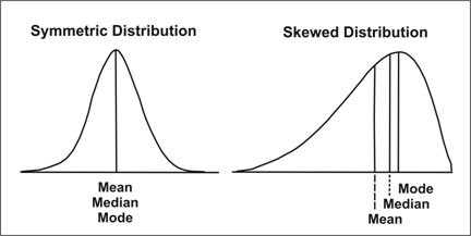
Measures of central location and spread are useful for summarizing a distribution of data. They also facilitate the comparison of two or more sets of data. However, not every measure of central location and spread is well suited to every set of data. For example, because the normal distribution (or bell-shaped curve) is perfectly symmetrical, the mean, median, and mode all have the same value (as illustrated in Figure 2.10). In practice, however, observed data rarely approach this ideal shape. As a result, the mean, median, and mode usually differ.
How, then, do you choose the most appropriate measures? A partial answer to this question is to select the measure of central location on the basis of how the data are distributed, and then use the corresponding measure of spread. Table 2.11 summarizes the recommended measures.
Table 2.11 Recommended Measures of Central Location and Spread by Type of Data
| Type of Distribution | Measure of Central Location | Measure of Spread |
|---|---|---|
| Normal | Arithmetic mean | Standard deviation |
| Asymmetrical or skewed | Median | Range or interquartile range |
| Exponential or logarithmic | Geometric mean | Geometric standard |
In statistics, the arithmetic mean is the most commonly used measure of central location, and is the measure upon which the majority of statistical tests and analytic techniques are based. The standard deviation is the measure of spread most commonly used with the mean. But as noted previously, one disadvantage of the mean is that it is affected by the presence of one or a few observations with extremely high or low values. The mean is "pulled" in the direction of the extreme values. You can tell the direction in which the data are skewed by comparing the values of the mean and the median; the mean is pulled away from the median in the direction of the extreme values. If the mean is higher than the median, the distribution of data is skewed to the right. If the mean is lower than the median, as in the right side of Figure 2.10, the distribution is skewed to the left.
The advantage of the median is that it is not affected by a few extremely high or low observations. Therefore, when a set of data is skewed, the median is more representative of the data than is the mean. For descriptive purposes, and to avoid making any assumption that the data are normally distributed, many epidemiologists routinely present the median for incubation periods, duration of illness, and age of the study subjects.
Two measures of spread can be used in conjunction with the median: the range and the interquartile range. Although many statistics books recommend the interquartile range as the preferred measure of spread, most practicing epidemiologists use the simpler range instead.
The mode is the least useful measure of central location. Some sets of data have no mode; others have more than one. The most common value may not be anywhere near the center of the distribution. Modes generally cannot be used in more elaborate statistical calculations. Nonetheless, even the mode can be helpful when one is interested in the most common value or most popular choice.
The geometric mean is used for exponential or logarithmic data such as laboratory titers, and for environmental sampling data whose values can span several orders of magnitude. The measure of spread used with the geometric mean is the geometric standard deviation. Analogous to the geometric mean, it is the antilog of the standard deviation of the log of the values.
The geometric standard deviation is substituted for the standard deviation when incorporating logarithms of numbers. Examples include describing environmental particle size based on mass, or variability of blood lead concentrations.1
Sometimes, a combination of these measures is needed to adequately describe a set of data.
EXAMPLE: Summarizing Data
Consider the smoking histories of 200 persons (Table 2.12) and summarize the data.
Table 2.12 Self-Reported Average Number of Cigarettes Smoked Per Day, Survey of Students (n = 200)
Number of Cigarettes Smoked Per Day
       0     0     0     0     0     0     0     0     0     0     0     0
       0     0     0     0     0     0     0     0     0     0     0     0
       0     0     0     0     0     0     0     0     0     0     0     0
       0     0     0     0     0     0     0     0     0     0     0     0
       0     0     0     0     0     0     0     0     0     0     0     0
       0     0     0     0     0     0     0     0     0     0     0     0
       0     0     0     0     0     0     0     0     0     0     0     0
       0     0     0     0     0     0     0     0     0     0     0     0
       0     0     0     0     0     0     0     0     0     0     0     0
       0     0     0     0     0     0     0     0     0     0     0     0
       0     0     0     0     0     0     0     0     0     0     0     0
       0     0     0     0     0     0     0     0     0     0     2     3
       4     6     7     7     8     8     9    10    12    12    13    13
      14    15    15    15    15    15    16    17    17    18    18    18
      18    19    19    20    20    20    20    20    20    20    20    20
      20    20    21    21    22    22    23    24    25    25    26    28
      29    30    30    30    30    32    35    40
Analyzing all 200 observations yields the following results:
Mean = 5.4
Median = 0
Mode = 0
Minimum value = 0
Maximum value = 40
Range = 0–40
Interquartile range = 8.8 (0.0–8.8)
Standard deviation = 9.5
These results are correct, but they do not summarize the data well. Almost three fourths of the students, representing the mode, do not smoke at all. Separating the 58 smokers from the 142 nonsmokers yields a more informative summary of the data. Among the 58 (29%) who do smoke:
Mean = 18.5
Median = 19.5
Mode = 20
Minimum value = 2
Maximum value = 40
Range = 2–40
Interquartile range = 8.5 (13.7–22.25)
Standard deviation = 8.0
Thus, a more informative summary of the data might be "142 (71%) of the students do not smoke at all. Of the 58 students (29%) who do smoke, mean consumption is just under a pack* a day (mean = 18.5, median = 19.5). The range is from 2 to 40 cigarettes smoked per day, with approximately half the smokers smoking from 14 to 22 cigarettes per day."
 Exercise 2.11
The data in Table 2.13 (on page 2-57) are from an investigation of an outbreak of severe abdominal pain, persistent vomiting, and generalized weakness among residents of a rural village. The cause of the outbreak was eventually identified as flour unintentionally contaminated with lead dust.
- Summarize the blood level data with a frequency distribution.
- Calculate the arithmetic mean. [Hint: Sum of known values = 2,363]
- Identify the median and interquartile range.
- Calculate the standard deviation. [Hint: Sum of squares = 157,743]
- Calculate the geometric mean using the log lead levels provided. [Hint: Sum of log lead levels = 68.45]
Table 2.13 Age and Blood Lead Levels (BLLs) of Ill Villagers and Family Members — Country X, 1996
| ID | Age (Years) | BLL† | Log10BLL |
|---|---|---|---|
| 1 | 3 | 69 | 1.84 |
| 2 | 4 | 45 | 1.66 |
| 3 | 6 | 49 | 1.69 |
| 4 | 7 | 84 | 1.92 |
| 5 | 9 | 48 | 1.68 |
| 6 | 10 | 58 | 1.77 |
| 7 | 11 | 17 | 1.23 |
| 8 | 12 | 76 | 1.88 |
| 9 | 13 | 61 | 1.79 |
| 10 | 14 | 78 | 1.89 |
| 11 | 15 | 48 | 1.68 |
| 12 | 15 | 57 | 1.76 |
| 13 | 16 | 68 | 1.83 |
| 14 | 16 | ? | ? |
| 15 | 17 | 26 | 1.42 |
| 16 | 19 | 78 | 1.89 |
| 17 | 19 | 56 | 1.75 |
| 18 | 20 | 54 | 1.73 |
| 19 | 22 | 73 | 1.86 |
| 20 | 26 | 74 | 1.87 |
| 21 | 27 | 63 | 1.80 |
| ID | Age (Years) | BLL† | Log10BLL |
|---|---|---|---|
| 22 | 33 | 103 | 2.01 |
| 23 | 33 | 46 | 1.66 |
| 24 | 35 | 78 | 1.89 |
| 25 | 35 | 50 | 1.70 |
| 26 | 36 | 64 | 1.81 |
| 27 | 36 | 67 | 1.83 |
| 28 | 38 | 79 | 1.90 |
| 29 | 40 | 58 | 1.76 |
| 30 | 45 | 86 | 1.93 |
| 31 | 47 | 76 | 1.88 |
| 32 | 49 | 58 | 1.76 |
| 33 | 56 | ? | ? |
| 34 | 60 | 26 | 1.41 |
| 35 | 65 | 104 | 2.02 |
| 36 | 65 | 39 | 1.59 |
| 37 | 65 | 35 | 1.54 |
| 38 | 70 | 72 | 1.86 |
| 39 | 70 | 57 | 1.76 |
| 40 | 76 | 38 | 1.58 |
| 41 | 78 | 44 | 1.64 |
? Missing value
Data Source: Nasser A, Hatch D, Pertowski C, Yoon S. Outbreak investigation of an unknown illness in a rural village, Egypt (case study). Cairo: Field Epidemiology Training Program, 1999.
References (This Section)
- Griffin S., Marcus A., Schulz T., Walker S. Calculating the interindividual geometric standard deviation of r use in the integrated exposure uptake biokinetic model for lead in children. Environ Health Perspect 1999;107:481–7.
Previous Page Next Page: Summary
Image Description
Figure 2.10
Description: In a symmetric distribution the mean, median, and mode are all located in the center of the x-axis. In a skewed distribution, the mean, median, and mode are not located together. If skewed to the right, the mean occurs to the left of the median; mode occurs to the right of the median. Return to text.
- Page last reviewed: May 18, 2012
- Page last updated: May 18, 2012
- Content source: