

Section 7: Measures of Spread
 ShareCompartir
Section 7: Measures of Spread
Spread, or dispersion, is the second important feature of frequency distributions. Just as measures of central location describe where the peak is located, measures of spread describe the dispersion (or variation) of values from that peak in the distribution. Measures of spread include the range, interquartile range, and standard deviation.
Range
Definition of range
The range of a set of data is the difference between its largest (maximum) value and its smallest (minimum) value. In the statistical world, the range is reported as a single number and is the result of subtracting the maximum from the minimum value. In the epidemiologic community, the range is usually reported as “from (the minimum) to (the maximum),” that is, as two numbers rather than one.
Method for identifying the range
- Step 1. Identify the smallest (minimum) observation and the largest (maximum) observation.
- Step 2. Epidemiologically, report the minimum and maximum values. Statistically, subtract the minimum from the maximum value.
EXAMPLE: Identifying the Range
Find the range of the following incubation periods for hepatitis A: 27, 31, 15, 30, and 22 days.
- Step 1. Identify the minimum and maximum values.
Minimum = 15, maximum = 31 - Step 2. Subtract the minimum from the maximum value.
Range = 31–15 = 16 days
For an epidemiologic or lay audience, you could report that “incubation periods ranged from 15 to 31 days.” Statistically, that range is 16 days.
Percentiles
Percentiles divide the data in a distribution into 100 equal parts. The Pth percentile (P ranging from 0 to 100) is the value that has P percent of the observations falling at or below it. In other words, the 90th percentile has 90% of the observations at or below it. The median, the halfway point of the distribution, is the 50th percentile. The maximum value is the 100th percentile, because all values fall at or below the maximum.
Quartiles
Sometimes, epidemiologists group data into four equal parts, or quartiles. Each quartile includes 25% of the data. The cut-off for the first quartile is the 25th percentile. The cut-off for the second quartile is the 50th percentile, which is the median. The cut-off for the third quartile is the 75th percentile. And the cut-off for the fourth quartile is the 100th percentile, which is the maximum.
Interquartile range
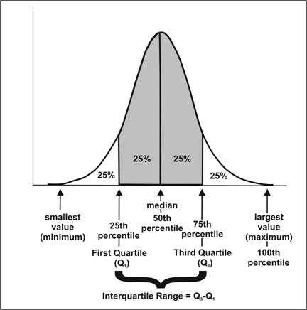
The interquartile range is a measure of spread used most commonly with the median. It represents the central portion of the distribution, from the 25th percentile to the 75th percentile. In other words, the interquartile range includes the second and third quartiles of a distribution. The interquartile range thus includes approximately one half of the observations in the set, leaving one quarter of the observations on each side.
Method for determining the interquartile range
- Step 1. Arrange the observations in increasing order.
- Step 2. Find the position of the 1st and 3rd quartiles with the following formulas. Divide the sum by the number of observations.
Position of 1st quartile (Q1) = 25th percentile = (n + 1) ⁄ 4
Position of 3rd quartile (Q3) = 75th percentile = 3(n + 1) ⁄ 4 = 3 × Q1 - Step 3. Identify the value of the 1st and 3rd quartiles.
- If a quartile lies on an observation (i.e., if its position is a whole number), the value of the quartile is the value of that observation. For example, if the position of a quartile is 20, its value is the value of the 20th observation.
- If a quartile lies between observations, the value of the quartile is the value of the lower observation plus the specified fraction of the difference between the observations. For example, if the position of a quartile is 20¼, it lies between the 20th and 21st observations, and its value is the value of the 20th observation, plus ¼ the difference between the value of the 20th and 21st observations.
- Step 4. Epidemiologically, report the values at Q1 and Q3. Statistically, calculate the interquartile range as Q3 minus Q1.
Figure 2.7 The Middle Half of the Observations in a Frequency Distribution Lie within the Interquartile Range
EXAMPLE: Finding the Interquartile Range
Find the interquartile range for the length of stay data in Table 2.8.
- Step 1. Arrange the observations in increasing order.
       0,      2,      3,      4,      5,      5,      6,      7,      8,      9,
       9,      9,     10,     10,     10,     10,     10,     11,     12,     12,
      12,     13,     14,     16,     18,     18,     19,     22,     27,     49
- Step 2. Find the position of the 1st and 3rd quartiles. Note that the distribution has 30 observations.
Position of Q1 = (n + 1) ⁄ 4 = (30 + 1) ⁄ 4 = 7.75Position of Q3 = 3(n + 1) ⁄ 4 = 3(30 + 1) ⁄ 4 = 23.25Thus, Q1 lies ¾ of the way between the 7th and 8th observations, and Q3 lies ¼ of the way between the 23rd and 24th observations.
- Step 3. Identify the value of the 1st and 3rd quartiles (Q1 and Q3).
Value of Q1: The position of Q1 is 7¾; therefore, the value of Q1 is equal to the value of the 7th observation plus ¾ of the difference between the values of the 7th and 8th observations:Value of the 7th observation: 6
Value of the 8th observation: 7Q1 = 6 + ¾(7−6) = 6 + ¾(1) = 6.75Value of Q3: The position of Q3 was 23¼; thus, the value of Q3 is equal to the value of the 23rd observation plus ¼ of the difference between the value of the 23rd and 24th observations:Value of the 23rd observation: 14
Value of the 24th observation: 16Q3 = 14 + ¼(16−14) = 14 + ¼(2) = 14 + (2 ⁄ 4) = 14.5 - Step 4: Calculate the interquartile range as Q3 minus Q1 .
Q3 = 14.5
Q1 = 6.75
Interquartile range = 14.5− 6.75 = 7.75
As indicated above, the median for the length of stay data is 10. Note that the distance between Q1 and the median is 10 − 6.75 = 3.25. The distance between Q3 and the median is 14.5−10 = 4.5. This indicates that the length of stay data is skewed slightly to the right (to the longer lengths of stay).
 Epi Info Demonstration: Finding the Interquartile Range
In the data set named SMOKE, what is the interquartile range for the weight of the participants?
What is the interquartile range of height of study participants? [Answer: 506 to 777]
Properties and uses of the interquartile range
- The interquartile range is generally used in conjunction with the median. Together, they are useful for characterizing the central location and spread of any frequency distribution, but particularly those that are skewed.
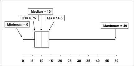
- For a more complete characterization of a frequency distribution, the 1st and 3rd quartiles are sometimes used with the minimum value, the median, and the maximum value to produce a five-number summary of the distribution. For example, the five-number summary for the length of stay data is:
Minimum value = 0,
Q1 = 6.75,
Median = 10,
Q3 = 14.5, and
Maximum value = 49. - Together, the five values provide a good description of the center, spread, and shape of a distribution. These five values can be used to draw a graphical illustration of the data, as in the boxplot in Figure 2.8.
Figure 2.8 Interquartile Range from Cumulative Frequencies
Some statistical analysis software programs such as Epi Info produce frequency distributions with three output columns: the number or count of observations for each value of the distribution, the percentage of observations for that value, and the cumulative percentage. The cumulative percentage, which represents the percentage of observations at or below that value, gives you the percentile (see Table 2.10).
Table 2.10 Frequency Distribution of Length of Hospital Stay, Sample Data, Northeast Consortium Vancomycin Quality Improvement Project
|
Length of Stay (Days)
|
Frequency
|
Percent
|
Cumulative Percent
|
|---|---|---|---|
| 0 | 1 | 3.3 | 3.3 |
| 2 | 1 | 3.3 | 6.7 |
| 3 | 1 | 3.3 | 10.0 |
| 4 | 1 | 3.3 | 13.3 |
| 5 | 2 | 6.7 | 20.0 |
| 6 | 1 | 3.3 | 23.3 |
| 7 | 1 | 3.3 | 26.7 |
| 8 | 1 | 3.3 | 30.0 |
| 9 | 3 | 10.0 | 40.0 |
| 10 | 5 | 16.7 | 56.7 |
| 11 | 1 | 3.3 | 60.0 |
| 12 | 3 | 10.0 | 70.0 |
| 13 | 1 | 3.3 | 73.3 |
| 14 | 1 | 3.3 | 76.7 |
| 16 | 1 | 3.3 | 80.0 |
| 18 | 2 | 6.7 | 86.7 |
| 19 | 1 | 3.3 | 90.0 |
| 22 | 1 | 3.3 | 93.3 |
| 27 | 1 | 3.3 | 96.7 |
| 49 | 1 | 3.3 | 100.0 |
| Total | 30 | 100.0 |
A shortcut to calculating Q1, the median, and Q3 by hand is to look at the tabular output from these software programs and note which values include 25%, 50%, and 75% of the data, respectively. This shortcut method gives slightly different results than those you would calculate by hand, but usually the differences are minor.
 Exercise 2.8
Determine the first and third quartiles and interquartile range for the same vaccination data as in the previous exercises.
2, 0, 3, 1, 0, 1, 2, 2, 4, 8, 1, 3, 3, 12, 1, 6, 2, 5, 1
Standard deviation
Definition of standard deviation
The standard deviation is the measure of spread used most commonly with the arithmetic mean. Earlier, the centering property of the mean was described — subtracting the mean from each observation and then summing the differences adds to 0. This concept of subtracting the mean from each observation is the basis for the standard deviation. However, the difference between the mean and each observation is squared to eliminate negative numbers. Then the average is calculated and the square root is taken to get back to the original units.
xxxxxxxxxxxxxxxxxxxxxxxxxxxxxxxxxxxxxxxxxxxxxxxxxxxxxxxxxx
Method for calculating the standard deviation
To calculate the standard deviation from a data set in Analysis Module:
Click on the Means command under the Statistics folder
In the Means Of drop-down box, select the variable of interest
→ Select Variable
Click OK
→ You should see the list of the frequency by the variable you selected. Scroll down until you see the Standard Deviation (Std Dev) and other data.
- Step 1. Calculate the arithmetic mean.
- Step 2. Subtract the mean from each observation. Square the difference.
- Step 3. Sum the squared differences.
- Step 4. Divide the sum of the squared differences by n − 1.
- Step 5. Take the square root of the value obtained in Step 4. The result is the standard deviation.
Properties and uses of the standard deviation
- The numeric value of the standard deviation does not have an easy, non-statistical interpretation, but similar to other measures of spread, the standard deviation conveys how widely or tightly the observations are distributed from the center. From the previous example, the mean incubation period was 25 days, with a standard deviation of 6.6 days. If the standard deviation in a second outbreak had been 3.7 days (with the same mean incubation period of 25 days), you could say that the incubation periods in the second outbreak showed less variability than did the incubation periods of the first outbreak.
- Standard deviation is usually calculated only when the data are more-or-less “normally distributed,” i.e., the data fall into a typical bell-shaped curve. For normally distributed data, the arithmetic mean is the recommended measure of central location, and the standard deviation is the recommended measure of spread. In fact, means should never be reported without their associated standard deviation.
EXAMPLE: Calculating the Standard Deviation
Find the mean of the following incubation periods for hepatitis A: 27, 31, 15, 30, and 22 days.
- Step 1. Calculate the arithmetic mean.
Mean = (27 + 31 + 15 + 30 +22) ⁄ 5 = 125 ⁄ 5 = 25.0 - Step 2. Subtract the mean from each observation. Square the difference.
Value Minus Mean Difference Difference Squared 27 − 25.0 + 2.0 4.031 − 225.0 + 6.0 36.015 − 225.0 −10.0 100.030 − 225.0 + 5.0 25.022 − 225.0 − 3.0 9.0 - Step 3. Sum the squared differences.
Sum = 4 + 36 + 100 + 25 + 9 = 174 - Step 4: Divide the sum of the squared differences by (n − 1). This is the variance.
Variance = 174 ⁄ (5 − 1) = 174 ⁄ 4 = 43.5 days squared - Step 5: Take the square root of the variance. The result is the standard deviation.
Standard deviation = square root of 43.5 = 6.6 days
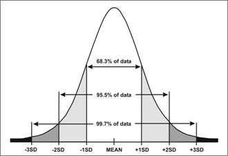
Areas included in normal distribution:
±1 SD includes 68.3%
±1.96 SD includes 95.0%
±2 SD includes 95.5%
±3 SD includes 99.7%
Consider the normal curve illustrated in Figure 2.9. The mean is at the center, and data are equally distributed on either side of this mean. The points that show ±1, 2, and 3 standard deviations are marked on the x-axis. For normally distributed data, approximately two-thirds (68.3%, to be exact) of the data fall within one standard deviation of either side of the mean; 95.5% of the data fall within two standard deviations of the mean; and 99.7% of the data fall within three standard deviations. Exactly 95.0% of the data fall within 1.96 standard deviations of the mean.
Figure 2.9 Area Under Normal Curve within 1, 2 and 3 Standard Deviations
Exercise 2.9
Calculate the standard deviation for the same set of vaccination data.
2, 0, 3, 1, 0, 1, 2, 2, 4, 8, 1, 3, 3, 12, 1, 6, 2, 5, 1
Standard error of the mean
Definition of standard error
The standard deviation is sometimes confused with another measure with a similar name — the standard error of the mean. However, the two are not the same. The standard deviation describes variability in a set of data. The standard error of the mean refers to variability we might expect in the arithmetic means of repeated samples taken from the same population.
The standard error assumes that the data you have is actually a sample from a larger population. According to the assumption, your sample is just one of an infinite number of possible samples that could be taken from the source population. Thus, the mean for your sample is just one of an infinite number of other sample means. The standard error quantifies the variation in those sample means.
Method for calculating the standard error of the mean
- Step 1. Calculate the standard deviation.
- Step 2. Divide the standard deviation by the square root of the number of observations (n).
Properties and uses of the standard error of the mean
- The primary practical use of the standard error of the mean is in calculating confidence intervals around the arithmetic mean. (Confidence intervals are addressed in the next section.)
EXAMPLE: Finding the Standard Error of the Mean
Find the standard error of the mean for the length-of-stay data in Table 2.10, given that the standard deviation is 9.1888.
- Step 1. Calculate the standard deviation.
Standard deviation (given) = 9.188 - Step 2. Divide the standard deviation by the square root of n.
n = 30
Standard error of the mean = 9.188 ⁄ √30 = 9.188 ⁄ 5.477 = 1.67
Confidence limits (confidence interval)
Definition of a confidence interval
Often, epidemiologists conduct studies not only to measure characteristics in the subjects studied, but also to make generalizations about the larger population from which these subjects came. This process is called inference. For example, political pollsters use samples of perhaps 1,000 or so people from across the country to make inferences about which presidential candidate is likely to win on Election Day. Usually, the inference includes some consideration about the precision of the measurement. (The results of a political poll may be reported to have a margin of error of, say, plus or minus three points.) In epidemiology, a common way to indicate a measurement’s precision is by providing a confidence interval. A narrow confidence interval indicates high precision; a wide confidence interval indicates low precision.
Confidence intervals are calculated for some but not all epidemiologic measures. The two measures covered in this lesson for which confidence intervals are often presented are the mean and the geometric mean. Confidence intervals can also be calculated for some of the epidemiologic measures covered in Lesson 3, such as a proportion, risk ratio, and odds ratio.
The confidence interval for a mean is based on the mean itself and some multiple of the standard error of the mean. Recall that the standard error of the mean refers to the variability of means that might be calculated from repeated samples from the same population. Fortunately, regardless of how the data are distributed, means (particularly from large samples) tend to be normally distributed. (This is from an argument known as the Central Limit Theorem). So we can use Figure 2.9 to show that the range from the mean minus one standard deviation to the mean plus one standard deviation includes 68.3% of the area under the curve.
Consider a population-based sample survey in which the mean total cholesterol level of adult females was 206, with a standard error of the mean of 3. If this survey were repeated many times, 68.3% of the means would be expected to fall between the mean minus 1 standard error and the mean plus 1 standard error, i.e., between 203 and 209. One might say that the investigators are 68.3% confident those limits contain the actual mean of the population.
In public health, investigators generally want to have a greater level of confidence than that, and usually set the confidence level at 95%. Although the statistical definition of a confidence interval is that 95% of the confidence intervals from an infinite number of similarly conducted samples would include the true population values, this definition has little meaning for a single study. More commonly, epidemiologists interpret a 95% confidence interval as the range of values consistent with the data from their study.
Method for calculating a 95% confidence interval for a mean
- Step 1. Calculate the mean and its standard error.
- Step 2. Multiply the standard error by 1.96.
- Step 3. Lower limit of the 95% confidence interval =
mean minus 1.96 × standard error.
Upper limit of the 95% confidence interval =
mean plus 1.96 × standard error.
EXAMPLE: Calculating a 95% Confidence Interval for a Mean
Find the 95% confidence interval for a mean total cholesterol level of 206, standard error of the mean of 3.
- Step 1. Calculate the mean and its error.
Mean = 206, standard error of the mean = 3 (both given) - Step 2. Multiply the standard error by 1.96.
3 × 1.96 = 5.88 - Step 3. Lower limit of the 95% confidence interval = mean minus 1.96 × standard error.
206 − 5.88 = 200.12
Upper limit of the 95% confidence interval = mean plus 1.96 × standard error.
206 + 5.88 = 211.88
Rounding to one decimal, the 95% confidence interval is 200.1 to 211.9. In other words, this study’s best estimate of the true population mean is 206, but is consistent with values ranging from as low as 200.1 and as high as 211.9. Thus, the confidence interval indicates how precise the estimate is. (This confidence interval is narrow, indicating that the sample mean of 206 is fairly precise.) It also indicates how confident the researchers should be in drawing inferences from the sample to the entire population.
Properties and uses of confidence intervals
- The mean is not the only measure for which a confidence interval can or should be calculated. Confidence intervals are also commonly calculated for proportions, rates, risk ratios, odds ratios, and other epidemiologic measures when the purpose is to draw inferences from a sample survey or study to the larger population.
- Most epidemiologic studies are not performed under the ideal conditions required by the theory behind a confidence interval. As a result, most epidemiologists take a common-sense approach rather than a strict statistical approach to the interpretation of a confidence interval, i.e., the confidence interval represents the range of values consistent with the data from a study, and is simply a guide to the variability in a study.
- Confidence intervals for means, proportions, risk ratios, odds ratios, and other measures all are calculated using different formulas. The formula for a confidence interval of the mean is well accepted, as is the formula for a confidence interval for a proportion. However, a number of different formulas are available for risk ratios and odds ratios. Since different formulas can sometimes give different results, this supports interpreting a confidence interval as a guide rather than as a strict range of values.
- Regardless of the measure, the interpretation of a confidence interval is the same: the narrower the interval, the more precise the estimate; and the range of values in the interval is the range of population values most consistent with the data from the study.
Demonstration: Using Confidence Intervals
Imagine you are going to Las Vegas to bet on the true mean total cholesterol level among adult women in the United States.
Exercise 2.10
When the serum cholesterol levels of 4,462 men were measured, the mean cholesterol level was 213, with a standard deviation of 42. Calculate the standard error of the mean for the serum cholesterol level of the men studied.
Image Description
Figure 2.7
Description: Bell-shaped curve. The central tendency, the middle is the median, 50th percentile. 25% to the left is the 25th percentile, the first quartile (Q1). 25% to the right of the median is the 75th percentile, the third quartile (Q3). The interquartile range goes from Q1 to Q3 and makes up 50% of the area under the curve. The largest value is the 100th percentile. Return to text.
Figure 2.8
Description: An Interquartile Range is depicted along a horizontal axis. The minimum is on the left followed by Q1, the median, Q3 and the maximum on the far right. Return to text.
Figure 2.9
Description: Bell-shaped curve with the standard deviations equally distributed on the x-axis. 99.7% of the data falls between the minus 3 and plus 3 standard deviation. 95.5% of the data falls between the minus 2 and plus 2 standard deviation. 68.3% of the data falls between the minus 1 and plus 1 standard deviations. Return to text.
- Page last reviewed: May 18, 2012
- Page last updated: May 18, 2012
- Content source: