

Module 5: Plot Standard Curves
 ShareCompartir
This module forms a fully annotated plot of the points contained in a standards data file along with the fitted standard curve. This module will access the coefficient data file to determine which fitting techniques were chosen during parameter estimation and only offer these for plotting. Thus, if only the robust fit was selected in Module 4, the user would not have the option of selecting unweighted least squares for plotting.
A nonparametric fit, the three point cubic spline, is also offered as an additional option which is always available for selection. The standard curve line described by the spline fit is programmed to pass through the median value of the replicate optical densities at each dilution along the curve. The user may enter this module prior to parameter estimation if it is desired to view the shape of the data in the standards data file before an attempt is made to fit the logistic-log function. In this case, the spline fit will be the only option available. In addition, if there were any plates in a standards data file where the solution did not converge to a stable set of parameter estimates after processing the data with Module 4, then the spline fit, again, will be the only option available for these plates.
These standard curve plots may be directed to the screen and any printer addressed through the Windows interface. The user may direct a single plot or an entire file of standard curve plots to the printer.
This module is entered from the main menu (Figure 3) and begins by displaying a standards data file selection dialog window. If the user enters this module directly after abstracting the data from a .DAT file (Module 3), or estimating the logistic-log parameters (Module 4), ELISA for Windows will insert a file name in the file name box which corresponds to the .DAT or .STD file just processed. This is offered as a convenience to the user in an attempt to eliminate repetitive entry of file names. This file is selected by clicking on OK. The user may also select a different file from the file list box.
After a standards data file has been chosen, the dialog window in Figure 15 appears. The window lists the name of the file and the number of plates contained in the file. The user should enter the desired plate in the appropriate text box. When the plate number field is exited, ELISA for Windows will interrogate the coefficient file associated with the standards data file and determine which types of fit should be made available for selection for that particular plate. Fits which were not used during parameter estimation will be suppressed as options here. If a coefficient file does not exist then the spline fit will be the only available option. As stated earlier, when a coefficient file does exist, the spline fit is the only method allowed for those plates where the solution did not converge during parameter estimation.
If the user selected the printer as the graph destinations, ELISA for Windows will display the plot on screen and then automatically send the screen image to the printer without user intervention. If the entire file is selected for processing, the printer is the only allowed destination. The user will be presented with all options for type of fit. If the program was unable to estimate coefficients for the standard curve for one or more of the plates in the file, the spline fit will automatically be chosen for these when they are displayed to the screen and sent to the printer. If the screen is selected as the destination for the graph, a plot will follow with the type of fit and standards file name appearing at the top of the screen. A typical plot will appear as shown in Figure 16. The 95% confidence intervals are included with the unweighted least squares fit. The user may scroll through the other standards series in the file by clicking on the Next and Previous buttons. Each plot may be directed to the printer at this stage. If the user elected to plot the entire file, each one will transmitted to the printer automatically, without user intervention.
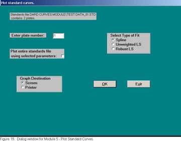
Figure 15. Dialog window for Module 5 – Plot Standard Curves.
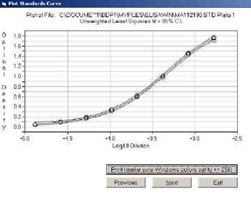
Figure 16. Typical plot of standard data overlaid with fitted standard curve.
- Page last reviewed: September 4, 2013
- Page last updated: September 21, 2005
- Content source: