

Module 4: Parameter Estimation
 ShareCompartir
Note: Although this software and accompanying documentation is dated 2004-2005, it is still valid in 2014. Questions can be sent to CDC-INFO.
This module uses a four parameter logistic-log function to describe standards data and form calibration curves. Standard curves may be formed using two fitting techniques, iteratively unweighted least squares and robust iteratively reweighted least squares. Users may also elect one of two estimation algorithms, Taylor series-linearization or Marquardt’s Compromise, to estimate the four parameters. It is beyond the scope of this document to describe these two techniques in detail. Briefly, the unweighted least squares method estimates the parameters without taking into account the possible differences in the variability of optical density measurements as one moves from dilution to dilution. Recognizing that this fit may be unduly influenced by aberrant observations (outliers), the robust fitting technique weights each observation individually and inversely proportionally to the residual difference between the observed and predicted values for each point. In this way, outliers are assigned low weights and exert little influence in the overall fit of the curve to the data.
Interested readers may refer to references 4 and 7 (listed at the end of this section) and to the Process Qualification Report for a further discussion of the theoretical details. Note that in their article, Tiede and Pagano refer to the four parameter function as a ‘modified hyperbola.’ In fact, it is algebraically equivalent to the logistic-log model. References 5 and 6 provide additional articles of interest. Our philosophy governing the use of these models in assay methodology is described in reference 1. For a discussion of the Taylor series-linearization and Marquardt’s Compromise estimation algorithm, readers are referred to Chapter 24, an Introduction to Nonlinear Estimation, in reference 2. Reference 3 describes the Marquardt’s Compromise technique in detail.
Users should be aware of the following broad generalizations when deciding which fitting algorithm to use:
- The Marquardt’s Compromise algorithm may, at times, expend more calculations, take more CPU time to arrive at a final set of estimates, and involve more iterations than does the Taylor series-linearization technique.
- The iterative steps tend to be smaller, especially as the converging process nears an end. However, this algorithm is more elaborate and is not as sensitive to poor starting values as the Taylor series technique.
- Marquardt’s Compromise is usually used when the Taylor series-linearization process fails to converge to a solution.
Since the model describing the standards data is the four parameter logistic-log function, a minimum of five data points is required for parameter estimation. Note that this does not mean there need be a minimum of five separate dilutions, just five data points spread out over some number of dilutions. Of course, if the data do not adhere to some semblance of a sigmoidal, S-shaped curve, this procedure will fail. It is the responsibility of the user to select a dilution schedule that will insure that there is enough information for ELISA for Windows to successfully estimate the four parameters.
A third fitting technique, the cubic spline, is also implemented in ELISA for Windows. This method is accessed directly in the ‘Plot Standard Curves’ (Module 5) and ‘Calculate Concentrations’ (Module 6) segments of the program and is discussed in further detail in those sections of this documentation. The spline fit is a useful technique in those cases where the parametric logistic-log function will not converge to a solution. This is often the case when the standards do not fully describe a sigmoidal-shaped curve. It is inherently difficult to arrive at reliable parameter estimates for the logistic-log function without a clear indication of the minimum and maximum optical densities associated with the assay. That is, if it is difficult to discern both lower and upper asymptotes for the sigmoidal-shaped curve (areas where the curve flattens out), then the logistic-log function fitting techniques may not converge to a solution. In this case, the spline fit may be used to interpolate antibody concentrations for unknown patient samples in Module 6.
Standards File Selection
This module is entered from the main menu (Figure 3) and begins by displaying a standards data file selection dialog window. If the user enters this module directly after abstracting the data from a .DAT file (Module 3), ELISA for Windows will insert a file name in the file name box which corresponds to the .DAT file just processed. This is offered as a convenience to the user in an attempt to eliminate repetitive entry of file names. This file is selected by clicking on OK. The user may also select a different file from the file list box.
Once the standards data file has been selected, ELISA for Windows responds with the dialog window shown in Figure 11.
The default selections in this dialog window include using the Marquardt’s compromise estimation algorithm with the robust fitting technique. All output will be directed towards the printer. The entire standards data file will be processed without interruption with each step using up to 100 iterations. The starting values for the iterative estimation process will be calculated by the program.
Users may alter these default settings to best handle their data sets. The estimation techniques are options and, as such, only one may be selected. The destination of the results are also options and users may select either the printer, computer screen, or file. If the screen is selected then the results of each plate are displayed on screen. Users then have the option of exiting to the next plate or printing the contents of the screen. If ‘file’ is selected, the user will be prompted for the name of a file to save the results. ELISA for Windows will suggest file.FIT, where file is the root file name of the standards data file. If the user selects the printer or file, the standards data will be processed without interruption with all output directed towards the printer or the designated file. The type of least squares fit are marked with check boxes. As such, robust, unweighted least squares, or both may be selected. If the user inadvertently neglects to select a type of fit, the robust fit is used as the default.
Coefficient Update
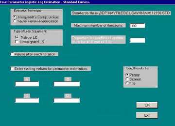
Figure 11. Dialog window for Module 4 – Parameter Estimation.
Users have the opportunity to enter the proportion for coefficient update. Note that this parameter is only valid when the Taylor series estimation algorithm is selected. If the Marquardt’s Compromise algorithm is chosen then this option is suppressed, as the Marquardt technique calculates the update factor automatically. This number must be greater than 0.0 and less than or equal to 1.0. We have found that the value 0.4 works well for our applications and is the default value which appears in the text box in the dialog window when the Taylor series estimation technique is selected. If desired, the user may alter this value. The program may occasionally fail to converge to a solution with some data sets. Outliers will severely affect the outcome of the algorithm used to calculate initial starting values for the iterative fitting procedure. In this case, coefficients from a previously successful run with similar data may be substituted for the calculated starting values and the iterative process retried. Alternatively, the proportion for the coefficient vector update can be modified. This is seen more clearly if one examines the weighted least squares equation:
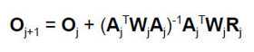
and re-expresses it as:
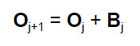
where
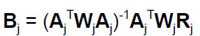
The most recent estimate for the parameter vector O = Oj+1 is equal to the last estimate, Oj, plus an amount equal to Bj. If Bj is very large the solution may circle around some value without actually converging, or it may rapidly expand and diverge to the point of causing a numeric overflow in the program. To avoid this, the magnitude of Bj may be decreased by altering the proportion for the coefficient vector update. If the user enters 1.0 then the result is the standard equations listed above. If the solution does not converge or if it diverges to numeric overflow, a smaller proportion, e.g. 0.4, may be used. This would modify the second equation, above, to:
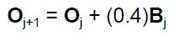
The proportion may be altered at will to compute smaller and smaller increments of change for the Oj vector. ELISA for Windows suggests a starting value of 0.4 and uses this as its default entry. The user is free to experiment with this value. Numbers close to 1.0 will result in larger steps between iterations and may lead to faster convergence (it may also lead to faster divergence as well). Numbers close to 0.0 will lead to smaller steps between iterations and lead to a slower convergence. This may be necessary for difficult data sets.
Number of Iterations
If the coefficient for vector update is small (less that 0.4), then the iterative increments tend to be smaller, requiring more steps to reach a stable set of coefficients. The default number of iterations is 100 and this may be increased to accommodate these situations. This is particularly true for those instances where the standards data do not fully describe a sigmoidal-shaped curve causing the iterative steps to proceed slowly to a final solution.
Note that the default setting for the number of iterations is set to 100. If the program is left unattended and loops around a solution, it will print out the results of the 100th iteration as though this were the final answer. Take care to examine the output. If the number of iterations is listed as 100 or 101, or, if the number is listed as that which was entered by the user, then the solution may be suspect. If this occurs, the user should examine the standards data as well as the fitted calibration curve using Module 5 – ‘Plotting Standard Curves’.
Pause after Iteration
The user may elect to view the results of each iteration by checking the ‘Pause after each iteration’ box. Coefficients with the resulting sum of squares of residuals and correlation coefficient are displayed on screen after each step of the fitting procedure. A general guideline as to whether or not a revised set of coefficients is performing better than the previous set is the sum of squares of the residuals which should decrease with each successive iteration. If the number steadily increases, this is an indication that the solution is starting to diverge. The program may still converge at a later stage or it may continue to diverge until a numeric overflow occurs. If it decreases then increases and starts to decrease again in a cyclic fashion, this is an indication that the program is circling around a solution without actually being able to achieve convergence.
It is important to note that there are two sums of squares of residuals returned for the approximate least squares fit and the robust fit. The regular sum of squares is simply the sum of the squared residuals. When fitting a simple linear model to a data set, this is the quantity that is minimized when solutions for the coefficients are found. In the case where a nonlinear function such as the four parameter logistic-log model is being fit using the Taylor series expansion method, an approximation to this quantity (the approximate sum of squares) is actually minimized when the coefficients are solved. As the solution converges, notice that these two quantities approach each other in magnitude. They should be fairly close to each other if the process concludes successfully. Interested users are referred to Chapter 24 of reference 2 – pages 508-511 for further details. In particular, equation 24.1.9 details the regular sum of squares of the residuals and equation 24.2.7 the approximation to this quantity resulting from the Taylor series expansion. Note the four coefficients change with smaller and smaller increments as they also converge to their final estimated values.
At the end of each iteration, ELISA for Windows will pause and display information as shown in Figure 12. If this particular iteration is satisfactory, and the user wishes to end the process, selecting ‘No’ will conclude the estimation process for the current plate, record the coefficients as detailed on screen, and proceed to the next plate. Selecting ‘Yes’ will initiate another iteration step. This process cycles until ELISA for Windows iterates to its own solution or the user stops the process by selecting ‘No’.
Estimation Starting Values
Good starting values are essential for the success of any nonlinear iterative fitting process. We have incorporated an algorithm which computes starting values for the iterative process used by ELISA for Windows to estimate the four parameters of the logistic-log function (see reference 4). Occasionally, these values will not lead to a solution, that is, the process will diverge away from a solution or circle around a solution without actually settling in on one set of values which may be used for parameter estimates. This is especially true if there are outliers in the data or if there are a small number of data points. ELISA for Windows gives the user the option of overriding the automatically calculated starting values so that a set of possibly more accurate values from a previously run standards file may be used in their place.
If the user elects to input starting values, the box for this option must be checked, otherwise, coefficient data entry will be suppressed. One or more starting values for coefficient estimation may then be entered. ELISA for Windows will insert the automatically calculated starting values in those instances where the user did not manually enter them. As an example, one may manually enter starting values for the first two coefficients (A and B) and leave the remaining coefficients (C and D) blank. The program will access the user inputted values for A and B and internally calculate values for C and D.
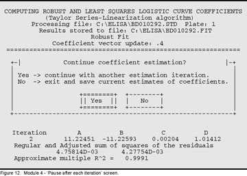
Figure 12. Module 4 – “Pause after each iteration” screen.
Solution Nonconvergence
ELISA for Windows, will complete process a standards data file even when one or more plates within the file contain data where coefficients may not be estimated. In those instances the output will be annotated with the message ‘Solution did not converge’ on the right side of the listing (described below). In this fashion the program will not end midstream while analyzing a standards file containing many plates. ELISA for Windows will keep track of those plates where convergence was not achieved. In succeeding modules, these situations are addressed by offering the spline fit as the only option for plotting standard curves or calculating antibody concentrations.
Analysis Strategies
Through the various options just outlined, an analysis strategy could proceed as follows: Select the Taylor series estimation technique with 0.4 for the proportion for the coefficient vector update. Choose the desired type of fit. The program will proceed through the selected type of fit for each set of standards in the .STD file.
There are a variety of strategies to employ if the program does not converge to a solution. If the starting values generated from ELISA for Windows‘s internal algorithm are distant enough from the true solution, the fitting procedure may not converge to a final set of values. Users should try the Marquardt’s Compromise algorithm if the Taylor series technique fails.
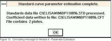
Figure 13. Concluding message for Module 4 – Parameter Estimation.
When the program fails to converge, the investigator should first try to select coefficients from a previously successful run with similar data and substitute them for the calculated starting values through the manual entry of starting values detailed previously. If such values are unavailable, the investigator should rerun the program choosing a smaller proportion for the coefficient vector update – say 0.3 or 0.2. As the program proceeds, the user should inspect the coefficients and the sum of squares of the residuals. The coefficients should stabilize and the sum of squares decrease.
If the solution does not converge but circles around a solution without actually converging, again, examine the sum of squares of the residuals that is returned after each iteration. The coefficients that return the smallest sum of squares can be used as starting values for another attempt at finding a solution. When re-executing the program, manually enter these coefficients and select a smaller proportion for the coefficient vector update than was used previously, and monitor the iterative process.
If the solution continues to circle around a set of values without actually converging, select those values which return the smallest sum of squares of the residuals and test them examining the goodness of fit statistics. If the error rates are acceptable, these coefficients may be used to form the standard curve. These results may also be examined graphically using Module 5, which produces a logistic-log plot.
Output Interpretation
Figure 14 contains an abbreviated listing of output generated from this module (Refer to page 52 for a sample of a complete listing). A complete listing for a sample data file is included in Appendix A. The logistic model used in ELISA for Windows is parameterized as:
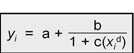
Where a = the upper asymptote of the sigmoidal curve, a + b = the lower asymptote, c is related to the dilution at the midpoint of the assay, and d is a curvature parameter, related to the slope of the curve; yi = the i th optical density and xi = thei th relative dilution (individual sample dilution / maximum dilution in the series) multiplied by 100.0. The output will list the file name of the standards file and the plate position within the file along with the type of fit, least squares or robust. Recall that a standards (.STD) file may include several plates of standards. Next the output will list the number of iterations required to reach a solution. Again, if this number is at the maximum set by the user, the results are suspect. ELISA for Windows simply stopped the iterative process after the maximum possible iterations and chose the last set of coefficients as the final set. The starting values for the coefficients used in the iterative process are listed next.
A table of values follows for each of the standards. The first column is the sample dilution. The second column is the relative dilution calculated as:
((sample dilution/maximum dilution) × 100).
The measured or known optical density occupies the third column followed by the predicted optical density from the fitted curve. The residual is calculated as: the known OD – predicted OD.
The % error equals the absolute value of:
(residual / known OD) × 100.0.
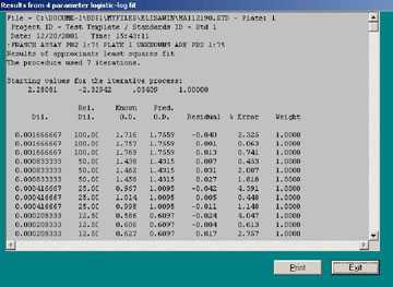
Figure 14. Sample output from Module 4 – Parameter Estimation.
Note that the % error may not precisely equal this quantity when performed on a hand-held calculator. This is due to roundoff error since ELISA for Windows performs most of these calculations in double precision and retains many more significant digits than are displayed in the output window. The weight column lists the individual weights used for the observation in the final fit of the logistic-log model to the data. For the least squares fit this weight will be set at 1.00 for all observations, indicating that each data point exerted equal influence in the final fit of the model to the data. This essentially is the result of an unweighted fit. For the robust fit, these weights will range from 0.0 to 1.0. The closer the weight is to 0.0, the less influence that point will exert on the fit. The points with weights closer to 1.0 will exert much more influence in the final fit than points with weights close to 0.0. Points with low weights may be considered potential outliers.The final estimates for the four coefficients follow in order of a, b, c, and d (refer to listing in Appendix A). The regular and adjusted sums of squares, as well as the approximate multiple R2 follow. For the least squares fit, the variances of the four coefficients are reported.
Typically, the window used to display the results will not be large enough to frame the entire listing. There are horizontal and vertical scroll bars on the bottom and right side of the window, respectively. Clicking the left mouse key on the down arrow of the vertical scroll bar will advance the listing one line. Clicking just above the arrow key will advance the listing by one screen. The horizontal scroll bar is used in the same manner to shift the listing left and right.
It should be noted that users may edit the contents of the output window. Comments may be added to further annotate the output. Several rudimentary Micro-soft Word operations will work in these windows. For example, text may be marked by clicking the left mouse key and dragging the cursor through the target text or pressing the shift key while moving the cursor through the text with the cursor control keys. Once text is marked it may be deleted, moved, etc.
After reviewing the contents of the output window, clicking on ‘Exit’ will erase the screen and proceed to the next round of estimation with a new plate or additional type of fit. Clicking on ‘Print’ will send the contents of the output window to the printer. If edits were made in the output window, these changes will be reflected in the printed outputs. They will not be saved once the user clicks on ‘Exit’.
References
- C. M. Black, B. D. Plikaytis, T. W. Wells, R. M. Ramirez, G. M. Carlone, B. A. Chilmonczyk and C. B. Reimer, Two-site immunoenzymometric assays for serum IgG subclass infant/mother ratios at full term, (1988) J. Immunol. Methods, 106:71-81.
- N. R. Draper and H. Smith, Applied Regression Analysis, third edition, (1998), John Wiley & Sons, Inc., New York.
- D. W. Marquardt, An algorithm for least squares estimation of nonlinear parameters, J. Society for Industrial & Applied Mathematics, (1963) 11:431-441.
- B. D. Plikaytis, G. M. Carlone, P. Edmonds, and L. W. Mayer, Robust estimation of standard curves for protein molecular weight and linear-duplex DNA base-pair number after gel electrophoresis, (1986) Anal. Biochem., 152:346-364. Erratum 154: 702 (1986).
- B. D. Plikaytis, P. F. Holder, L. B. Pais, S. E. Maslanka, L. L. Gheesling, and G. M. Carlone, Determination of Parallelism and Nonparallelism in Bioassay Dilution Curves, (1994) J. Clin. Microbiol, 32:2441-2447.
- B. D. Plikaytis, S. H. Turner, L. L. Gheesling, and G. M. Carlone, Comparisons of standard curve-fitting methods to quantitate Neisseria meningitidis Group A polysaccharide antibody levels by enzyme-linked immunosorbent assay, (1991) J. Clin. Microbiol., 29:1439-1446.
- J. J. Tiede and M. Pagano, The application of robust calibration to radioimmunoassay, (1979) Biometrics 35:567-574.
- Page last reviewed: September 4, 2013
- Page last updated: September 21, 2005
- Content source: