Chapter Six. User Manual with Example

In this chapter, we provide an example of how to use the web tool and illustrate its features. The tool allows users to change five broad parameters: the state, the list of interventions to analyze, the analysis type (cost-effectiveness or portfolio), the run type (with or without fines and fees), and budget. This example uses only one state, but the parameters are the same for all states. Finally, we show how the sensitivity analysis works; this is available only with portfolio analysis.

Figure 6.1 shows the home page. From the home page, a new user would probably want to proceed to the introduction for an explanation of the various features of the web tool. Repeat users can skip the introduction and proceed to one of the two types of analysis, the basic cost-effectiveness analysis or the portfolio analysis, by selecting a state from the drop-down menu, clicking the button next to the desired analysis, and clicking Submit. Some users may want to use the library, which contains reports providing detailed information about the input data, assumptions, and methodology. After leaving the home page, the user can navigate through the tool using the menu in the upper left corner of the screen.

Figure 6.1. Screenshot of the Home Page

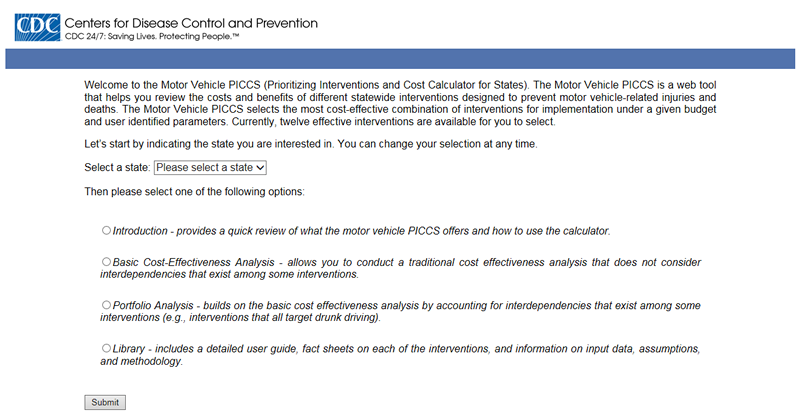
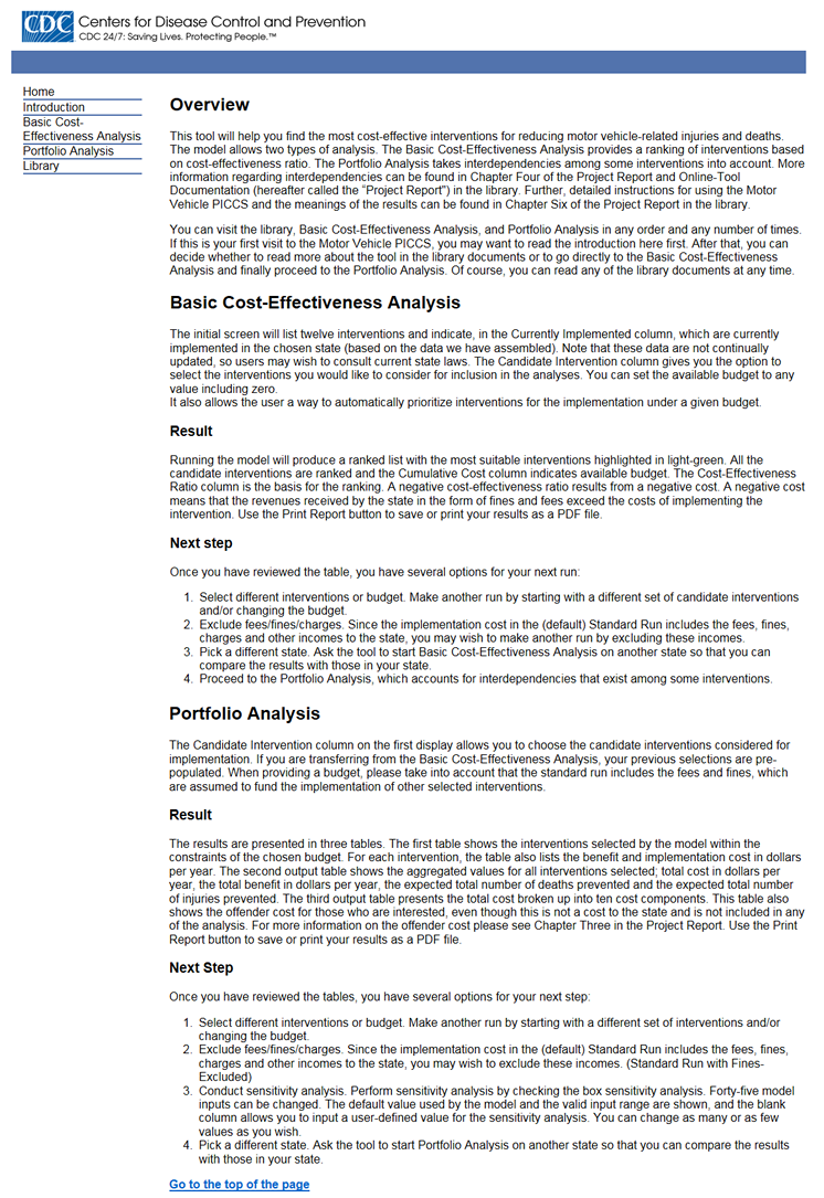
Figure 6.2 shows the introduction, which briefly explains how to use either cost-effectiveness analysis or portfolio analysis.

Figure 6.2. Screenshot of the Introduction

For the examples in this section, we use Georgia. We start with a basic cost-effectiveness analysis. On the opening page (shown in Figure 6.1), the user selects Georgia from the drop-down menu of states, selects Basic Cost-Effectiveness Analysis, and clicks Submit. Figure 6.3 shows the initial cost-effectiveness analysis page, with Georgia selected as the state for analysis. In the top table, the first two columns show that all interventions are selected (this is the default), while the second column indicates those that are already implemented in Georgia.³³ The third column ranks the interventions in the order of their cost–effectiveness ratio, and the fourth column shows the names of the interventions. The fifth and sixth columns show the estimated effectiveness and costs per year, and the seventh column shows the cumulative cost as each intervention is added to the preceding ones. The last two columns show the annual reductions in deaths and injuries. The footnote text appears on each screen; we have included it in Figure 6.3 but deleted it from subsequent figures.

Figure 6.3. Screenshot of Sample Basic Cost-Effectiveness Analysis for Georgia, Input Screen

For our example, we deselect three of the interventions that Georgia already has in place (primary enforcement seat belt law, bicycle helmets, and sobriety checkpoints) and keep the other 11 interventions for inclusion in the analysis. The user does this by deselecting the box associated with the intervention in the first column. Interventions with checks in the first column will be included in the analysis. The user is not required to deselect the interventions that are already in place and can leave them in to see what effect they have or if the user believes that the information about the current implementation status is incorrect. In many cases, a state may have an intervention in place, but it is not fully implemented. In this case, a user might choose to include that intervention in the analysis to see what the costs and effects of full implementation would be.

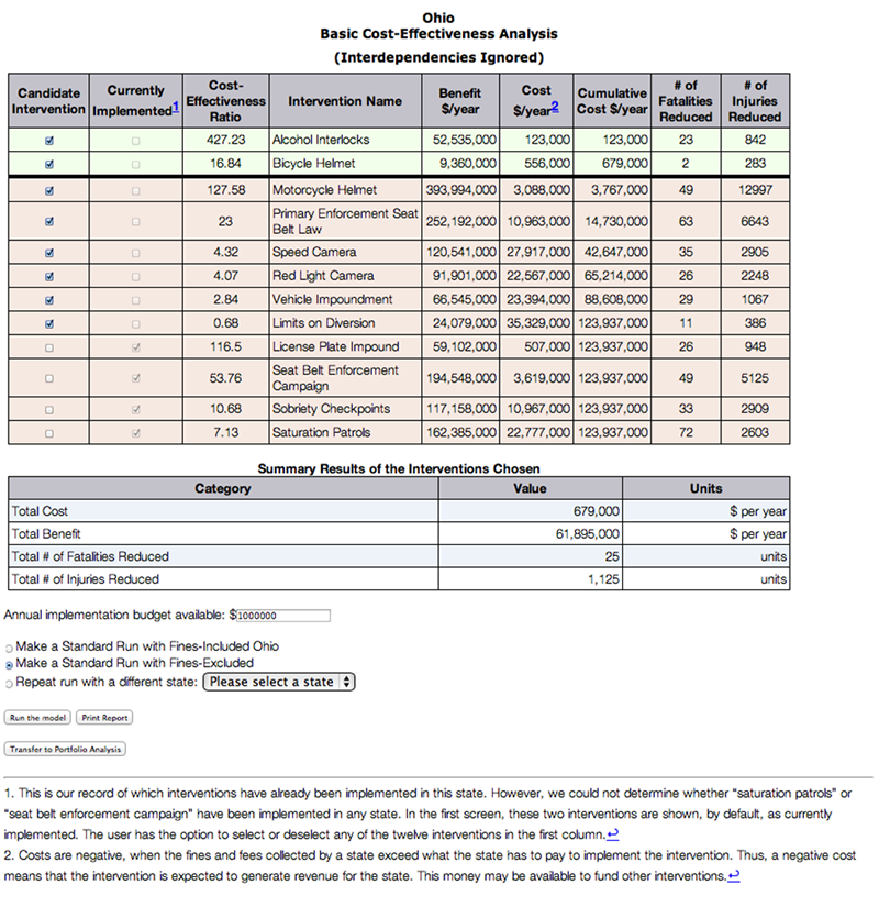
Beneath the summary result table is a box in which the user can set the annual implementation budget and select the run type. For this example, we make a run with fines excluded, so that button is selected. Because this means that no fine or fee revenues can defray the costs of implementation, we also add a budget of $10 million^.34 We then click Run the model. The results of this analysis are shown in Figure 6.4.

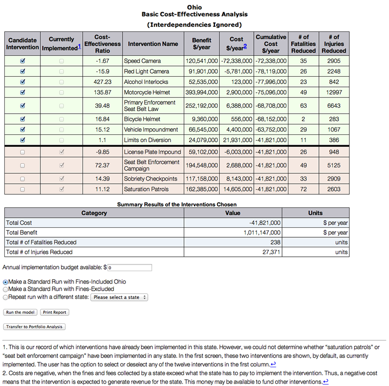
Figure 6.4. Screenshot of Sample Basic Cost-Effectiveness Analysis for Georgia, Fines Excluded and $10 Million Budget

Of the 11 interventions selected for analysis, six are shown in green and five in pink, separated by a bold line. This means that the given budget of $10 million can cover the implementation of six interventions. The total cost of these six is $5.6 million, which is within our budget. (The row with the last intervention that the tool selected—that is, the last green row—will always equal the summary cost because this is the cumulative total of all selected interventions.) Four of the five interventions in pink exceed $10 million, so the tool does not select those; the fifth, saturation patrols, costs $8.1 million but has a far lower cost-effectiveness ratio than those that were selected.³⁵ If we include increased seat belt fines for analysis, the tool will always select it because the cost of implementation is $0 (see “Higher Seat Belt Fine” under “Intervention Cost Estimate Assumptions” in Chapter Three for an explanation). These six interventions together save 212 lives and prevent 24,963 injuries.

For the next run, we retain these 11 interventions for analysis and include fines and fees. In the tool, we can do this by changing the radio button from Make a Standard Run with Fines-Excluded to Make a Standard Run with Fines-Included. We leave the budget at $10 million and run the model.

Figure 6.5. Screenshot of Sample Basic Cost-Effectiveness Analysis for Georgia, Fines Excluded, $10 Million Budget

Now the tool selects all 11 interventions. In the Cost $/year column, we see that the speed-camera intervention has negative $71.9 million in costs because of the collection of fines that provide revenue to the state.³⁶ If we add to this the fine and fee revenue from three other interventions that also have negative costs (increased seat belt fines, red-light cameras, and license plate impoundments), this is a total of $86.4 million available to defray the implementation costs. We can also see that the cost for some other interventions has declined as well; for example, motorcycle helmet laws had a cost of $1.86 million in Figure 6.4 and a cost of $1.76 million in Figure 6.5. This is because some fines and fees are collected from offenders, but the cost is still positive because the revenues do not cover the full cost of implementation.

Assuming that the revenues can be used for implementing other interventions, the $86.4 million that these interventions generate provides sufficient revenues to fund all 11 interventions. As can be seen in the summary results table, the state still gains roughly $65.7 million even if it implements all 11 interventions. The $10 million budget that the state provides would not be needed in this case. These 11 interventions also prevent 33,968 injuries and 368 deaths annually. Monetizing the potential loss from these injuries and deaths means that the interventions produce a collective benefit of more than $1.15 billion.³⁷

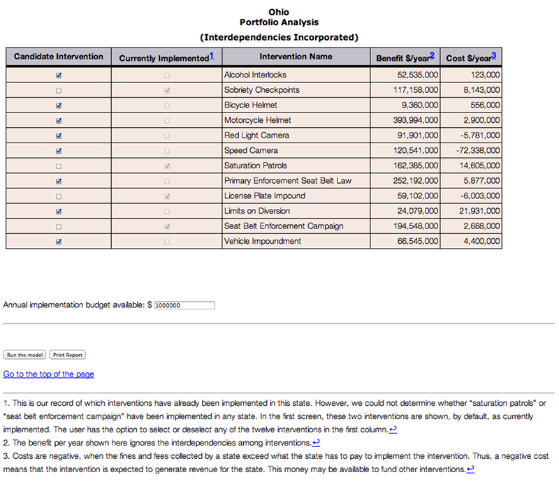
To illustrate how the portfolio analysis works, we use the same example. We select Transfer to Portfolio Analysis from the options at the bottom of the screen. The initial screen is shown in Figure 6.6. This screen is a streamlined version of the initial screen for standard analysis. The selection of interventions remains in the far left column. When the user arrives at this screen from a cost-effectiveness analysis, all the previously selected interventions remain selected.

Figure 6.6. Screenshot of Sample Portfolio Analysis for Georgia, Input Screen

At the bottom of the table, we retain the previous budget of $10 million per year. We then select Run the model. This initial portfolio analysis run is always a standard run with fines included.

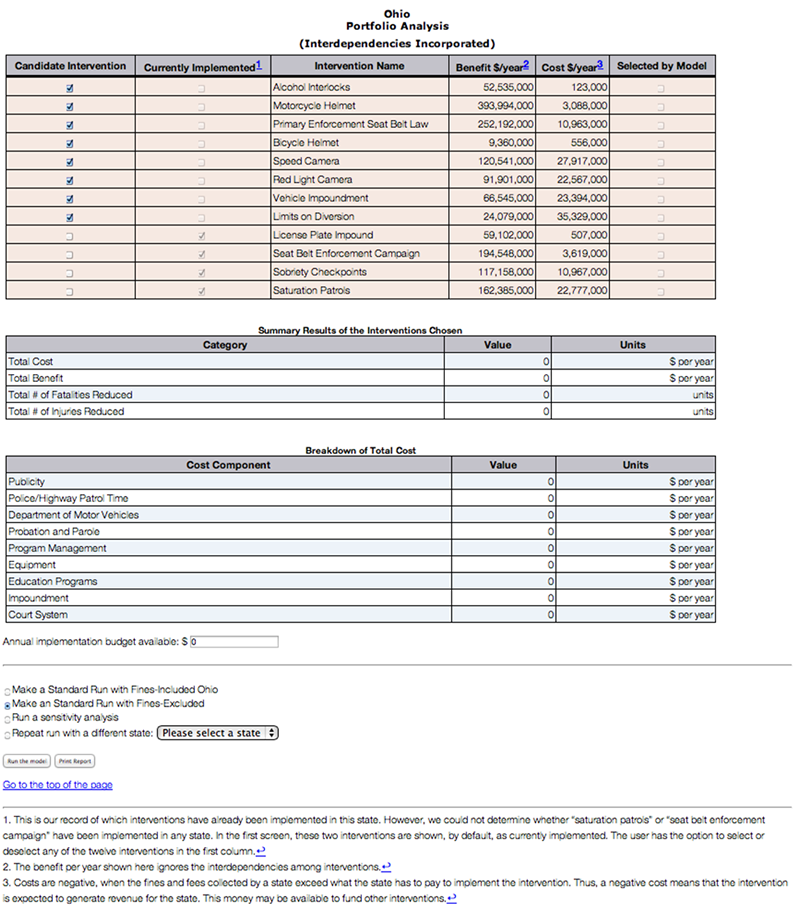
The results of this run are shown in Figure 6.7. As with the similar run in the cost-effectiveness analysis (see Figure 6.5), the model selects all 11 interventions. Again, the revenue provided by the fines from the speed-camera, red-light camera, increased seat belt fine, and license plate impoundment interventions, if allocated to other interventions, would allow all interventions to be funded. As the summary table shows, the revenue to the state is the same as with the cost–effectiveness ratio analysis, about $65.7 million annually.

In the cost-effectiveness analysis, funding all 11 interventions resulted in an estimate of 33,968 injuries prevented and 368 lives saved, for a monetized savings of about $1.15 billion annually (Figure 6.5). However, that analysis does not take into account the interdependencies of the various interventions and therefore double-counts some of the effectiveness. This problem is avoided in the portfolio analysis (Figure 6.7), in which the 11 interventions have slightly lower effectiveness: 32,754 injuries and 343 deaths prevented and a monetized annual benefit of about $1.09 billion.³⁸

Generally speaking, the total cost in cost-effectiveness and portfolio analysis should be the same, although rounding the numbers occasionally results in a slight difference. There is one exception: If more than one seat belt intervention is included, the costs are adjusted slightly downward because their implementation costs overlap.

The “Breakdown of Total Cost” table shows the ten cost components. The first ten lines sum to the total cost line in the summary table. Two lines of the ten will always be negative or zero. “Fines and Fees” includes all monies that offenders pay to the state, so this is revenue to the state and shown as negative. This line could be zero if the only selected interventions were among the three that do not carry any fines or fees (alcohol interlocks, bicycle helmets, and in-person license renewal). “Education Programs” will likewise always be negative or zero because our cost assumption is that the fee that an offender required to take a class pays is higher than the cost that the state pays to provide the class.

This table also includes two additional lines that are not included in the total costs. “Offender-Borne Cost” shows costs that offenders pay but not to the state, such as the cost of having a private company install an alcohol interlock. “Cost to Comply with the Law” is the sum of the costs that individuals pay to avoid violating laws, such as the cost to purchase a motorcycle or bicycle helmet. Table 3.2 in Chapter Three shows all four types of costs: state costs, state revenues (paid by individuals to the state), offender-borne costs, and costs to comply with the law.

Figure 6.7 Screenshot of Sample Portfolio Analysis for Georgia, Fines Included, $10 Million Budget

It is also possible to run sensitivity analysis for the portfolio analysis. The sensitivity analysis allows the user to change many of the key input values. If we select Run a sensitivity analysis and then click the Run the model button, the sensitivity analysis portion is shown in Figures 6.8 and 6.9. (Note that the sensitivity run defaults to a model run that includes fines and fees. In this case, because we just did this type of run, the output table is identical to that in Figure 6.7). There are 45 inputs (the relevant injury-to-fatality ratios, injury reductions, state-adjusted costs, fatality reductions, and implementation costs) and the model’s default selections (“Default Value”) for each. The user can substitute a value for any or all of these inputs.³⁹ For example, if the user has information about a difference between estimated injuries and deaths for a particular intervention, he or she can override the tool’s current use of proportional estimates and assign different estimates to each.

Figure 6.8. Screenshot of Sensitivity Analysis Table Inputs for Sample Portfolio Analysis for Georgia, Fines Included, $10 Million Budget, Part 1 of 2

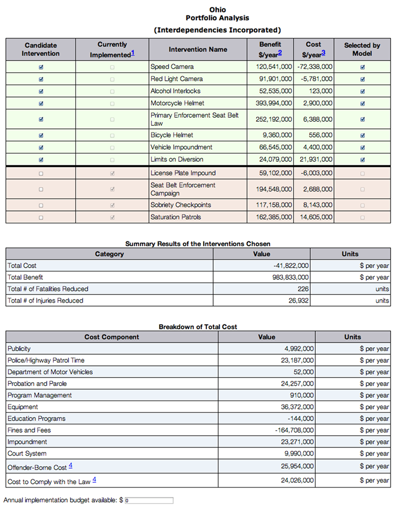
Figure 6.9. Screenshot of Sensitivity Analysis Table Inputs for Sample Portfolio Analysis for Georgia, Fines Included, $10 Million Budget, Part 2 of 2

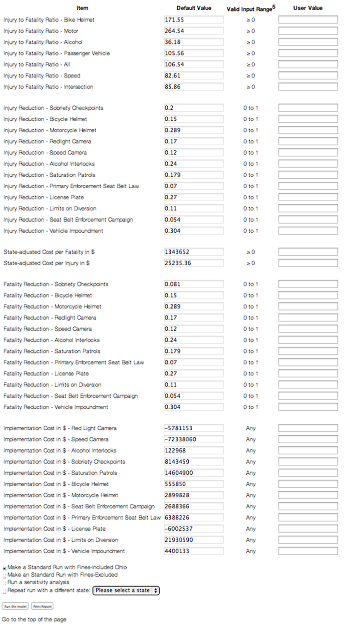
For our example, we change the annual implementation cost for speed cameras from –$72.9 million to $0 and for red-light cameras from –$6 million to $0, to test what happens if the state sets fines from automated enforcement equal to costs such that the program covers its own costs but nothing more. We then click Run the model to get the results. This is still a standard run with fines included, 11 interventions selected, and an annual implementation budget of $10 million.

The results of the run are shown in Figure 6.10. Despite not having the funds available from the speed and red-line cameras and a $10 million annual implementation budget, the model now selects ten interventions shown in green at the top of the upper table. The removal of limits on diversion means that the number of injuries and deaths prevented has decreased slightly. The funds come from the fines generated by the license plate impoundment and increased seat belt fines, along with the $10 million budget.

The “Breakdown of Total Cost” table now excludes the costs associated with the limits on diversion because the tool did not select that intervention. However, this table does not reflect the changes to the speed and red-light camera costs because the sensitivity analysis does not break down any changes to total cost for an intervention into its individual cost components.

Figure 6.10. Screenshot of Sample Portfolio Analysis with Sensitivity Analysis for Georgia, Fines Included, $10 Million Budget, $0 in Speed-Camera and Red-Light Camera Fines Collected

At the bottom of each page is a Print Report button, which generates a printer-friendly PDF of the current analysis.

The user can move from state to state in two ways: selecting the radio button for Repeat run with a different state or going back to the home page.

 

Footnotes

33. Although saturation patrols and seat belt enforcement campaign are not shown as already implemented, their actual status is not known according to our assembled record of state laws. The user should first provide the status for each by leaving it checked in the second column if it has been implemented or by checking it in the first column if it has not been implemented. 
34. All budget figures must be entered as numerals with no spaces or dollar signs. 
35. The increase seat belt fine intervention always has a cost-effectiveness ratio of 0 because there is no cost. 
36. As noted in Chapter Five, fines are displayed as a negative cost, because they constitute revenue to the state.
37. This benefit does not include the net cash flow of $65.7 million from the cost side.
38. In addition to being more accurate, portfolio analysis can serve other purposes. First, it can be used to see whether the simpler cost–benefit ratio analysis serves as a good approximation. Second, when each intervention can be funded at different levels but produces benefits at different degrees correspondingly, cost–benefit ratio analysis can break down and portfolio analysis is a much better approach. 
39. For background on choosing values for sensitivity runs, review different values, such as minimum, most common, and maximum, discussed in Chapter Three.