


Application of the ILO International Classification of Radiographs of Pneumoconioses to Digital Chest Radiographic Images
 ShareCompartir
July 2008
DHHS (NIOSH) Publication Number 2008-139
Go back to Workshop Index page.
A NIOSH Scientific Workshop
DISCLAIMER: The findings and conclusions in these proceedings are those of the authors and do not necessarily represent the official position of the National Institute for Occupational Safety and Health (NIOSH). Mention of any company or product does not constitute endorsement by NIOSH. In addition, citations to Web sites external to NIOSH do not constitute NIOSH endorsement of the sponsoring organizations or their programs or products. Furthermore, NIOSH is not responsible for the content of these Web sites.
Image presentation: Implications of Processing and Display
Michael J. Flynn, PhD
Radiology Research
Henry Ford Health System
One Ford Place, Suite 2F
Detroit MI, 48202
Voice: 313-874-4483
FAX: 313-874-4494
Email: mikef@rad.hfh.edu
I. Introduction
For traditional film-screen (FS) radiography systems, the intensity of the radiation beam transmitted through the subject is directly transformed to film optical density and displayed with an illuminator. The display characteristics of a FS image cannot be altered after the radiograph has been acquired. For digital radiography (DR) systems, the recorded image is first stored temporarily as an array of raw image values and then transformed into presentation values that are used to display the image on an electronic device (see Figure 1). The visual characteristics of a DR image can be significantly improved by adjusting the brightness in light and dark regions, by enhancing detail contrast, by restoring blurred edges, and by reducing noise. Furthermore, the characteristics of the displayed image are also influenced by the transfer characteristics of the display system used for presentation. The influence of processing and display variables on the classification of pneumoconiosis in chest radiographs is considered in this paper.
II. Display Processing
Display processing methods perform the same function for all types of digital radiography detectors. The detector first produces raw image values that have a simple, usually linear or logarithmic, relationship to the input radiation intensity. Subsequently, display enhancement processes modify these data to restore sharpness, reduce the appearance of quantum noise, and increase detail contrast. The modified data can be mapped to standardized presentation values that are used by a calibrated display device to generate the image. The specific processing methods used in current systems are described in this paper.
IIa. Display Processing: Raw Image Data Values
For most computed radiography (CR) and flat panel DR systems, at each image position, the detector produces an electronic charge that is monotonically related to the radiation energy absorbed. At this stage, the signal (charge) can be considered as a function of the incident radiation exposure, S = k1 Kin. The system’s preamplifier and digital converter transform the charge to an integer representing the raw data image value, Iraw. A variety of instrument corrections are then applied to the raw image values to obtain values suitable for image processing, IQ. These include corrections to interpolate bad pixels and to adjust for non-uniformity.
Most systems transform the charge signal to a value proportional to the logarithm of the input exposure. Logarithmic signals have the property that a fractional change in S, due to the contrast of adjacent structures, produces a fixed change in the raw image value, DIQ, independent of subject penetration and input exposure. However, no medical or industry standards currently exist to define the scale of numbers used for raw image signal in digital radiographs. Systems may use logarithmic or square root transformations, and different vendors vary with respect to the constants used for the transformation. The final draft of the American Association of Physicists in Medicine Task Group 116, for publication in 2008, includes a recommendation for normalized For Processing values that are logarithmically related to exposure under standardized conditions, QK = 1,000*log10(KSTD/Ko) when KSTD is in microgray units, Ko = 0.001 μGy, and KSTD > Ko.
The wide variation in input signal transformations used by different vendors has hindered the introduction of consistent processing methods that can be applied at a workstation to images from various image acquisition products. Industry adoption of the new standardized values in conjunction with storage using the DICOM For Processing digital radiographic object should permit consistent results from secondary processing of radiographs submitted by different systems. In this chapter, display processing is illustrated using For Processing image data in a logarithmic value representation of the type described in the example above.
IIb. Display Processing: Grayscale Rendition
For Processing digital radiographic image data can have a range of values, depending on exposure factors ( kVp, mA-S, and filtration) and subject content (body part, body position, size, anatomy, pathology, and view). The highest signal intensities are found in regions outside of the subject where the direct beam is recorded. For chest radiographs, the lowest values are in regions below the diaphragm. Other anatomic regions are distributed with signal intensities ranging between these limits (see Figure 2).
In general, the grayscale rendition process maps the image values for anatomic regions that absorb the most radiation to the largest presentation values, for display at maximum brightness. Anatomic regions that absorb the least radiation are mapped to the smallest presentation values for display at minimum brightness. Intermediate image values are then mapped to presentation values in a monotonically decreasing fashion. This produces a presentation with a black background and white bones similar to that of conventional FS radiographs.
To emphasize the contrast of intermediate image values, the values of IQ are mapped to presentation values, Ip , using a non-linear relationship that emulates the Huerter-Driffeld curve (H-D curve) familiar from FS radiography. The maximum and minimum raw image values are extended and the intermediate values produce higher contrast than the extreme values. As with FS systems, the grayscale rendition may have an extended toe or shoulder to extend contrast into anatomic regions with low or high penetration. The values of Ip are defined with the expectation that the luminance response of the display, L(Ip), is calibrated to follow a standardized gray scale display function (GSDF). For film printers, Ip is related to film density such that when the film is placed on a viewer, the brightness will follow the standard GSDF. The commonly used DICOM GSDF produces similar contrast perception over the full range of brightness (2).
For electronic presentation using a PACS workstation, the raw For Processing image values may be sent along with DICOM header elements that indicate the minimum and maximum values of interest for presentation, i.e., the VOI LUT window width and window level elements (2). However, if For Presentation image data are sent to the workstation with a non-linear grayscale already applied, the ability of the observer to make further adjustments of image contrast and brightness is limited. Instead, images can be sent to a PACS station as raw image values along with a grayscale value of interest lookup table, i.e. the VOI LUT sequence (3).
Problems can arise if the same grayscale rendition is used to print films as is used to display images on an electronic display. This results from the extended density range of printed film, typically 0.12 OD to 3.2 OD, in relation to the more limited range of luminance for display monitors, typically 350-1. With film, dense regions are viewed using bright spot illuminators, whereas with review on a workstation the highly penetrated regions are viewed using adjustments to the grayscale rendition. This must be considered in protocols for standardized classification of radiographs.
IIc. Display Processing: Exposure Recognition
Exposure recognition processes are used to identify the minimum and maximum IQ values to be used for the grayscale rendition. In cases where the overall exposure to the image acquisition device is unusually high or unusually low, the histogram of IQ values will be shifted accordingly. When IQ is determined using a logarithmic transformation, a fractional change in the exposure level shifts the histogram a fixed amount. For example, if the exposure is doubled, the histogram may shift to the right by +301, whereas if the exposure is reduced by a factor of 2, the histogram may shift to the left by -301. If the desired range of IQ values can be identified for an individual image acquisition, the grayscale characteristics of displayed images can be similar, even if exposure variations shift the histogram.
Exposure recognition processes typically segment the signals due to anatomic regions from those recorded directly with no tissue attenuation or from areas that are outside the collimated radiation beam. Within the identified anatomic regions, intelligent algorithms then identify zones which should be displayed with maximum and minimum brightness. Segmentation may be aided by examining the noise characteristics of the image values and by identifying structures that have straight edge characteristics (4-6). Complex rules may be used to refine the segmentation and reduce errors to less that 1% of the cases (7). Once segmented, the correct range of IQ values is determined from the image values in the anatomic region. For views such as the PA chest, assumptions regarding the positions of the lung fields and mediastinum can be used; however, more complex approaches are required in general (8). These exposure recognition processes are analogous to the automatic exposure control systems used with modern photographic cameras. Like photographic camera products, many different approaches are employed on different DR products.
Another function of the exposure recognition process is to estimate the average radiation exposure to the receptor in the anatomic regions of interest. This is commonly reported to the operator as an index number that can be used to indicate whether the proper radiographic technique was used. CR systems made by Fuji Medical Systems report a number, S, which is inversely proportional to exposure1. CR systems made by Agfa Medical Systems report a number, lgM, which is proportional to the log of the exposure2. The lgM value varies with the user-selected speed, Sn. CR systems made by Eastman Kodak Company report an exposure index, EI, proportional to the log of the exposure3. Similar values are reported for the DR systems made by Eastman Kodak Company.
Unfortunately, the exposure index values used by different manufacturers vary in both scale and direction in relation to exposure. A primary objective of the American Association of Physicists in Medicine Task Group 116 reported referred to above was to make recommendations on a standardized exposure indicator for digital radiography. An international standard with similar definitions has recently been drafted and will be considered this year, IEC 62B/680/CDV. The adoption of common exposure indicators will make it easier to define protocols for standardization of radiographic studies.
IId. Display Processing: Edge Restoration
The x-ray projection through patient tissues that is recorded by a digital radiography detector depicts fine detail with some blur. Blur can be related to the x-ray tube focal spot, patient motion, or the detector (described by the modulation transfer function, MTF(f) of the device). Edge restoration processes are used to transform the blurred radiograph such that the fine detail better reflects the actual attenuation characteristics of the tissue structures. Since the detector MTF(f) is generally the dominant source of blur, increasing the spatial frequencies in the recorded image in proportion to 1/MTF(f) provides a better indication of the actual spatial frequency content of the tissue structures. In practice, unfortunately this can also produce a large increase in the high spatial frequency content and result in excessive amplification of quantum noise.
To limit noise amplification, edge restoration filters may principally amplify image components with low and intermediate spatial frequencies. As frequencies increase beyond the intermediate range, the 1/MTF(f) filter function slowly returns to values of 1 or less. The Metz filter was developed for this purpose and has been shown to be effective in improving radiographic observer performance (10). The filter can be varied to control the amount of high frequency gain permitted (11). Similar shapes can be obtained by modifying the inverse MTF(f) filter with a Butterworth filter that gradually diminishes coefficients above a specified frequency.
Edge restoration of this type can only be performed with knowledge of the MTF(f) for the detector system. Of particular importance is the reduction in modulation transfer that can occur at low and intermediate frequencies (i.e. from about .1 to .5 of the limiting frequency associated with the spacing of the image values). For CR systems using powdered phosphor screens, MTF(f ) is diminished at intermediated frequencies with f1/2 equal to about 1.2 cycles/mm for MTF(f) = 0.5 (13). For Cesium Iodide flat panel detectors, the value of f1/2 is slightly higher but a significant reduction in MTF(f) still occurs at mid frequencies. For detectors using photoconductors such as Selenium, the MTF(f) is more appropriately described by the ideal response of a square detector element, MTF(f) = sinc(pDx f) (14).
When the edge restoration filter is appropriately specified, fine detail has a realistic appearance and the image will not have excessive noise. This is illustrated in figure 3 for a lateral knee view recorded using a CR system with a high-resolution phosphor screen. Inappropriate specification of the restoration filter can lead to artifacts. In some systems of earlier design, filters were implemented using spatial convolutions based on a small kernel that were not able to amplify image components with low and intermediate spatial frequencies. These were often applied with excessively high gain. This over-amplification of high spatial frequencies causes edge artifacts appearing as an oscillating signal that is sometimes referred to as ‘edge ringing’.
If similar appearances are sought for images acquired from multiple medical centers as a part of a standardized classification protocol, it is important to recognize that edge restoration processes may need to be different, depending on whether the type of device that acquired the radiograph was a CR systems, indirect DR systems, and direct DR systems. However, important differences in appearance are not likely to results from using the same processing on devices of the same system type from different manufacturers.
IIe. Display Processing: Noise Reduction
All digital radiographic devices are designed such that the only visible noise is due to the limited number of x-rays detected per unit area. For photoconductive flat panel devices, the quantum noise appears with a very fine texture. The spatial frequency components of this noise are distributed with equal strength at all spatial frequencies, i.e. the noise power spectrum, NPS(f), is constant in relation to frequency (14). For detectors using scintillation phosphors, either CR or flat panel, the noise appears as a more nodular texture with the higher frequency components somewhat diminished in strength (13). In both cases, the relative noise amplitude of Idet is largest when the input exposure is small. For systems using logarithmic transformation, this causes the absolute noise amplitude in IQ to vary as the tissue attenuation varies in different regions of the image.
A variety of processing methods can be used to reduce the visual appearance of the noise texture. In general these methods all reduce the high frequency components associated with the noise signal resulting in a more nodular texture with reduced amplitude. As a consequence, these processes will also reduce the high frequency components of the tissue signal, resulting in some increased blur. A general aim of noise reduction processes is to reduce the noise only in regions where the tissue contrast does not have noticeable fine detail.
If the frequency content of the tissue contrast is known along with the frequency content of the noise, the frequency dependant contrast to noise ratio can be used to develop a noise reduction filter. The classical Wiener filter (15,16) provides an optimal solution based on the power spectrum of the tissue contrast signal, however it is not applicable when the signal and noise vary in the image. Adaptive noise reduction processes attempt to locally filter the image in regions where the tissue contrast has little fine detail. In regions containing sharp edges, fine detail, or other structures producing high frequency components, the noise reduction is constrained and the detail preserved. Methods that have been used in commercial systems include the Lee filter (17), adaptive Wiener filtering (18), and noise coring (26). Noise reduction processes are difficult to successfully implement since the goals of reducing noise and preserving resolution can conflict.
The ability of noise reduction techniques to improve visual performance has been the subject of much debate. Because the human visual system can effectively recognize target patterns in the presence of noise, it is not necessarily true that a reduction in noise amplitude will improve detection performance. Moreover, if the noise texture is made coarser and the filtered noise has a power spectrum similar to the target objects, the noise reduction process may be deleterious. This can be of particular concern when considering the fine texture of lung tissue and pneumoconiosis pathology in the chest radiograph.
IIf. Display Processing: Contrast Enhancement
Traditional FS radiographs with large latitude have poor contrast. This problem is of particular significance for chest radiography. If it is considered to be diagnostically important to visualize the contrast of lung tissue behind the mediastinum, behind the heart, or around the curved dome of the diaphragm, a wide latitude film-screen system is required and tissues in the primary lung region are recorded with flat contrast.
For digital radiography, contrast enhancement processes are able to greatly improve the contrast of local tissue structures without altering the global grayscale characteristics of the image. Image processing methods are used that maintain the low spatial frequency components of the image that are responsible for the average brightness in large regions while increasing the components with intermediate and high frequency that are responsible for detail contrast. Contrast enhancement processes result in both high contrast and wide latitude in a manner that is not possible with FS radiography.
The classical approach for contrast enhancement is the un-sharp mask method. A blurred representation of the image is first prepared. This is then subtracted from the image to reveal the detail contrast. The two are then combined with appropriate weighting to obtain an enhanced image (see Figure 4). The method originated as a photographic process where a blurred negative is placed in contact with a positive film to diffusely increase the light transmission in dark regions. A high contrast copy of the film is then made. This method has been commonly used to prepare prints for publication4 and was described in 1981 as a method to improve chest radiographs (19).
Fuji Medical Systems introduced unsharp mask processing of digital radiographs on their early CR systems (20, 21). Using appropriate weighting to diffusely increase low Iraw values and decrease high values, the range of values is compressed allowing the use of a narrow latitude grayscale rendition. The method is referred to as dynamic range control (DRC); however, the purpose is to permit increased contrast. Numerous enhancements to this method have subsequently been reported and are used in commercial systems (22-25). These approaches use varying numeric methods to obtain good control of the enhancement response in relation to spatial frequency.
The appearance of contrast enhanced images is dependent on the specific approach applied, in relation to spatial frequency affects, particularly at boundaries which have a large change in the attenuation. At such boundaries, all methods produce an artifact with a gradual short-range shift in image values. This response can be considered in terms of the shape of a convolution kernel used to blur the original image to obtain an unsharp mask (see Figure 5a). Early methods used large size kernels (1 to 4 cm) having constant values that caused a linearly varying transition at edges (see Figure 5b). The frequency response for such a kernel has an undesirable oscillating response that can cause excessive amplification of certain tissue patterns. In comparison, if the kernel values are derived from a Gaussian function, the frequency response monotonically increases in a well-behaved manner (see Figure 5c). Modern methods use multi-scale and multi-frequency processing methods that can be rapidly applied to achieve a well behaved enhancement (27, 28).
III. Display Presentation
Images that have been processed and are ready to be displayed will have values that are intended for presentation, Ip. These values are appropriately communicated in the DICOM digital radiography For Presentation object. Within a medical center with central storage facilities for medical imaging, these images would be retrieved by a computer workstation and displayed on a monitor that has been calibrated for the display of medical For Presentation image values. With proper calibration, the appearance of the image will be the same for any workstation. The calibration must consider the luminance response (grayscale) as well as the luminance ratio as described below.
IIIa. Display Presentation – graphic controller and monitor
Modern computer work stations utilize graphic controllers to convert image values to brightness, more formally luminance, for which the SI unit is candelas/m2. For modern liquid crystal display (LCD) devices, digital values are sent to the monitor where they are stored to control the brightness signal for each discrete pixel in the panel. For cathode ray tube (CRT) devices, an analog voltage signal was sent that controlled the electron beam current in real time as the beam was swept in a raster pattern. The CRT devices produced a blurred image and were subject to analogue signal drift which affected image contrast. As a consequence, current standardized protocols for digital radiography for which images are to be interpreted on workstations should avoid CRT devices.
The graphic controller converts the image values to the digital driving levels (DDL) of the computer monitor. Commonly this is done as a red, green, and blue (RGB) signal with 8 bits (256 levels) per channel. New standards are anticipated that will communicate more color levels to the monitor (10 to 16 bits). For the gray levels important in digital radiography, a variety of methods exist to communicate 256 or 1024 gray levels, each of which can be precisely defined from a palette with several thousand values. These more sophisticated methods are used in the graphic controllers and specialized calibration software designed for medical imaging. The transformation of For Presentation image values to the set of desired gray levels is done through a look up table (LUT). Determining and installing the LUT is the process that calibrates the display device.
IIIb. Display Presentation – Luminance Ratio
For a specific calibration LUT, the ratio of the luminance associated with the maximum gray level, Lmax, to the luminance of the minimum gray level, Lmin, is known as the calibrated luminance ratio, LR = Lmax/ Lmin. When a person is viewing a particular image, the eye and neuronal vision systems adapt to the overall scene brightness. The perception of contrast, as measured by the relative luminance change of a just visible target structure, is best when the target is located in a region of the image having a luminance equal to the adapted luminance (see figure 6). In brighter and darker portions of the image, the perception of contrast is diminished. If LR is too large, contrast in the very bright and very dark regions can become imperceptible. On the other hand, if LR is too small, the overall scene contrast is poor. An appropriate compromise is about 350, although values from 250 to 500 are used.
It is important to realize that if an image is viewed on a device with a specific LR, say 250, and later the image is viewed at a different LR, say 450, the appearance of the image will be significantly different. For chest radiographs at high LR, contrast is poorly demonstrated in the dark lung regions. This is conceptually illustrated in figure 7. For standardization of viewing conditions in multi-center reading, it is important that all display devices be calibrated to the same LR.
IIIc. Display Presentation – Luminance Response (grayscale).
The luminance in relation to the digital driving level is referred to as the luminance response, which is often called the grayscale response. The grayscale establishes the display contrast transfer characteristics in the various regions of an image that will be in dark, mid-gray, and bright areas of the scene. The native luminance response of a typical LCD monitor is poorly suited for displaying digital radiographs (see figure 8). A dark region with no contrast is followed by a rapid increase in brightness. For the mid driving levels and higher, the luminance is high with low contrast. This characteristic is well suited for general purpose computer graphic applications but not for medical or photographic images.
The DICOM committee defined a Grayscale Standardized Display Function (GSDF) that has been widely adopted by medical imaging manufacturers (2). This functions provides a modest boost in contrast at dark levels where human visual contrast response is not as good. Devices used for the presentation of digital radiographs should be calibrated to follow the GSDF between Lmin and Lmax. This is done through generation of the appropriate LUT which usually requires a luminance meter, although some equipment is sold with a predetermined LUT stored within the monitor.
IIId. Display Presentation – Device requirements
To assure standardization for consistent and accurate image classification, methods must be in place to ensure calibration of electronic display devices. Additionally, devices must have sufficient brightness, small pixel pitch, and good reflective properties. Room lighting should be low enough that the ambient luminance Lamb (in Lux), measured from the monitor surface with the monitor power off, is much less than Lmin. The human visual basis for the desired requirements are not detailed here (29, 30), but appropriate requirements can be summarized as;
- GSDF luminance response with LR = 350.
- Maximum brightness of 450 candelas/m2 or more
- Pixel pitch of 0.210 mm or less.
- Diagonal size of 20-24 inches with 4:3 or 5:4 aspect
- Lamb less than 1/4th of Lmin.
IIIe. Display Presentation – Film Prints
Digital radiographs may be printed on transparent sheet film to be viewed on traditional view-box illuminators, although this process may not be readily available, since many facilities prefer to send images using standardized digital formats on computer disks (CD). If prints are made, it is difficult to print a digital image with an appearance similar to an electronic display. For a device calibrated for LR = 350, the corresponding optical density range is about 2.5. Typically OD ranges for film printers are about 3.1. Thus the grayscale rendition needs to be adjusted to cover a wider range of image values to achieve similar appearance. This can be a particular problem in printing digitally-acquired chest images, in that the lungs can appear unusually dark.
IV. Discussion
When done properly, digital radiography processing can produce significant improvements in image quality compared to FS techniques. However, modern processing methods can also produce image characteristics that are different than the traditional FS appearance. As a consequence, most manufacturers can adjust the manner in which processing is applied. For a reader with little experience viewing processed digital images, an approach may be taken that mimics traditional film-screen appearance. For readers with more experience viewing digital images, a more aggressive approach to processing may be selected. This creates problems when trying to standardize the classification of pneumoconiosis patterns using images from many centers.
The following should be considered for future programs involving digital radiography with electronic viewing for the classification of the pneumoconioses:
- Consider a program requiring that radiographs be acquired and communicated using normalized For Processing values in DICOM standard format. If achieved, the following can be considered;
- Adoption of a NIOSH image processing engine that can be applied on a workstation to achieve a standardized appearance.
- Implementation of a processing service whereby For Processing data is sent to NIOSH for conversion to For Presentation images that are then sent to qualified readers for interpretation.
- In the absence of standards for normalized processing values,
- Utilize a chest phantom to qualify centers doing chest radiography
- Specify the general characteristics of the processing to be applied with illustrations.
- Require examples of processed images to be submitted as a part of the approval process.
- Where possible, indicate the nominal processing parameters that are to be applied for different manufacturers and software versions.
- For B readers, communicate images electronically using DICOM standards and require a reader display device certification, including
- Documentation of the device and its characteristics (see section IIId.)
- Review of quality control image(s) on the monitor and demonstration of the visibility of specified findings.
- Periodically verify the luminance calibration, potentially requiring the sending of a device and software to perform the verification.
Acknowledgement
Portions of the material contained in this report appeared in an RSNA course booklet on “Advances in Digital Imaging” that was published in 2003.
Figures
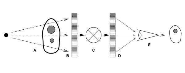
Figure 1. The examination of patients with digital radiography is illustrated as a six component model; A) generation of a beam of x-rays incident on the patient, B) modulation of the x-ray beam intensity by tissue structures, C) detection of the transmitted x-ray beam and creation of an array of raw image values ( Iraw ), D) transformation of Iraw values to presentation values ( Ip ) by display processing, E) display of the image with a standardized grayscale, and F) psycho-visual interpretation of the displayed image by the observer.
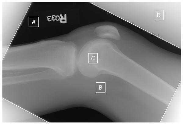
Figure 2a. Commonly observed regions are identified on an image of raw values, Iraw, from a knee radiograph; A) regions where the x-ray beam directly exposes the detector with no tissue attenuation, B) regions of modest tissue attenuation, C) regions of high attenuation from bone, and D) regions outside of the collimator edges exposed by scattered radiation.
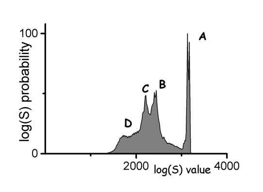
Figure 2b. A histogram of raw image values from a knee radiograph with commonly observed regions identified; A) direct exposure produces a narrow peak of high values, B) soft tissue regions produce a broad peak of values less than A, C) bone regions produce a broad peak of values less than B, and D) a diffuse peak of low values outside of the collimated region.
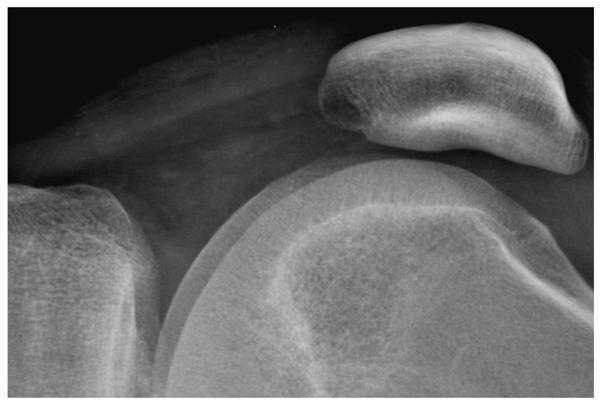
Figure 3a. A digital radiograph of the knee taken with a high resolution CR screen (HR screen, Eastman Kodak Company) is illustrated using display processing with no edge restoration.
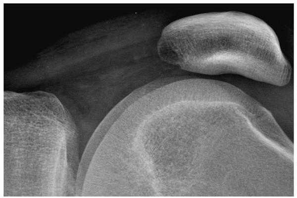
Figure 3b. The knee radiograph shown in figure 3a is illustrated using display processing with edge restoration.
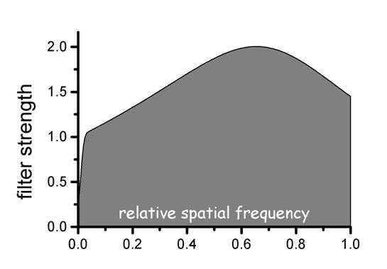
Figure 3c. The filter strength in relation to spatial frequency is shown for the edge processing used in figure 3b. Intermediate spatial frequencies are enhanced proportional to the inverse of the modulation transfer function (MTF). The inverse MTF filter is reduced at high spatial frequencies using a low pass Butterworth filter.
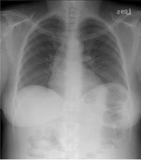
Figure 4a. A digital radiograph of the chest taken with a general purpose CR screen (GP screen, Eastman Kodak Company) is illustrated using no display processing. To display the wide range of raw image values, a wide latitude grayscale rendition has been used that results in poor tissue contrast.
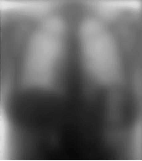
Figure 4b. An unsharp mask image derived from the chest image in figure 4a is illustrated with the grayscale reversed.
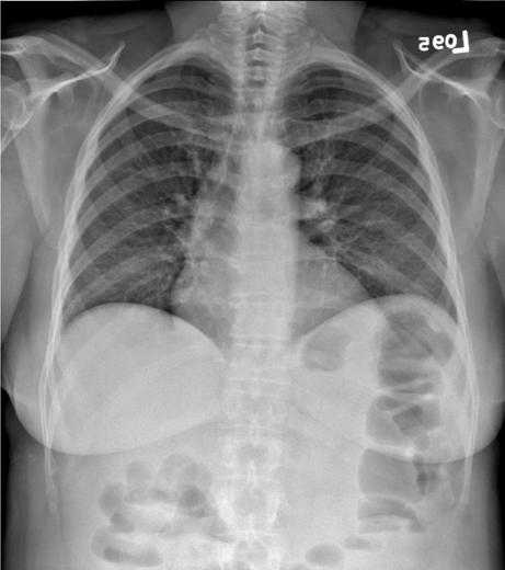
Figure 4c. The chest image in figure 4a is illustrated with contrast enhancement based on the unsharp mask of figure 4b. The unsharp mask values are used to adjust the raw image values so that the image may be displayed with a narrow latitude grayscale rendition resulting in improved tissue contrast. An equivalent photographic process would use the unsharp mask as illustrated to illuminate the orginal radiograph and make a high contrast copy.
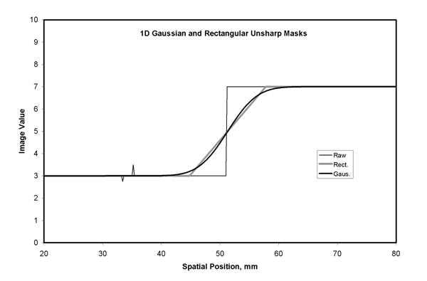
Figure 5a. Blurring of raw image values to obtain an unsharp mask is illustrated with a one dimensions (1D) line of data crossing a sharp edge. A rectangular smoothing kernel (Rect, 16 mm width) with constant kernel weights produces a linear transition at the edge. A Gaussian smoothing kernel (Gaus, 16 mm width at .27 of the maximum) produces a smoothly varying transition. The fine detail structures seen in the raw data on the left do not appear in the unsharp mask data.
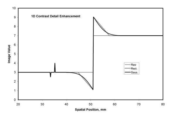
Figure 5b. Detail contrast enhancement based on an unsharp mask can be scaled so that the resulting image has the same values for low frequency components (i.e. the same latitude) but the contrast of edges and fine detail are amplified. This is illustrated using the 1D unsharp mask example from figure 5a. Note the smoothly varying overshoot at the edge that results from a Gaussian kernel (Gaus.). The detail contrast enhancement of the fine detail at the left is about 2 times that seen in the original data (see figure 5a).
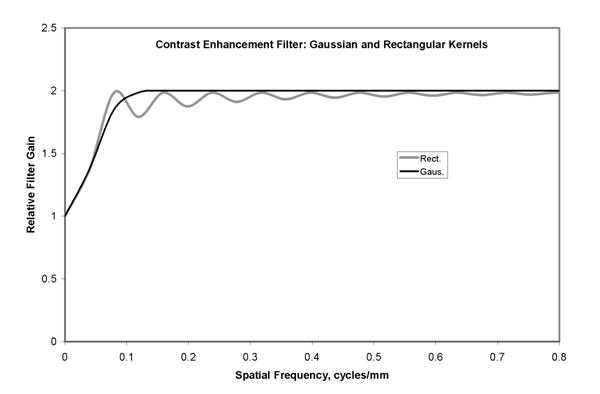
Figure 5c. The enhancement of image components as a function of spatial frequency is illustrated for the two examples of figure 5b. Using scaling to preserve latitude, the very low frequencies are amplified with a gain near 1.0. Amplication increases with frequency to a gain of 2.0 in order to enhance detail contrast. For the process with the rectangular kernel (Rect.), ringing of the amplification is seen. In comparison, the process with the Gaussian kernel (Gaus.) produces amplification that varies smoothly with spatial frequency.
Figure 6. The contrast threshold is a psycho-visual measure of human vision based on the just noticeable contrast, measured as luminance change divided by mean luminance. It is typically made using grating patterns with sinusoidal luminance variation at a particular spatial frequency. If the target and background are of the same average luminance and the average luminance is changed for each measure, the result is for varied adaptation. If the background is kept at constant luminance, and the average luminance of the target is varied, the result is for fixed visual adaptation.
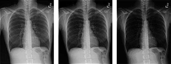
Figure 7. The appearance of the same image display with different display luminance ratios is simulated. At the left is the image presented with the desired luminance ratio. As the ratio is increased from left to right, the tissue structures in the lung become dark and contrast is not visible.

Figure 8. The native luminance response of a modern liquid crystal display, LCD, monitor is illustrated by the response of 6 devices of the same manufacturer and model. The luminance for a set of 1786 progressively increasing gray levels show abrupt increases in the low palette index range and poor contrast in the high index values. This type of response provides bright images for general purpose computer graphic images such as word processors, but provides poor rendering of medical or photographic images.
Figure 9. The DICOM Gray Scale Display Function, GSDF, provides a relationship between the Digital Driving Levels, DDL, of a display, and luminance. The values are tabulated in relation to an index, the Just Noticeable Difference index, whose spacing is proportional to the DDL levels.
References
- Shepard J, Wang J, Flynn M, Gingold E, Goldman L, Krugh K, Mah E, Ogden K, Peck D, Samei E, Willis C: An exposure indicator for digital radiography: Report of Task Group 116, American Association of Physicists in Medicine, Draft 9b, Nov 2007.
- Digital Imaging and Communications in Medicine (DICOM) Part 14: Grayscale Standard Display Function. National Electrical Manufacturers Association, Rosslyn VA, 2003.
- Digital Imaging and Communications in Medicine (DICOM) Part 3: Information Object Definitions. National Electrical Manufacturers Association, Rosslyn VA, 2003.
- Barski LL, Van Metter R, Foos DH et.al. New automatic tone scale method for computed radiography. In: SPIE Proceedings 1998, 3335: 164-178.
- Luo J and Senn R. Collimation for digital radiography. In: SPIE Proceedings 1997, 3034:74-85.
- Senn R and Barski L. Detection of skin line transition in digital medical imaging. In: SPIE Proceedings 1997, 3034:1114-1123.
- Dewaele P, Ibison M and Vuylsteke P. A trainable rule-based network for irradiation field recognition in Agfa’s ADC system. In: SPIE Proceedings 1996, 2708:72-84.
- Takeo H, Nakajima N, Ishida N, et.al. Improved automatic adjustment of density and contrast in FCR system using neural network. In: SPIE Proceedings 1994, 2163:98-109.
- Gur D, Fuhman CR, Feist JH, Slifko R, Peace B. Natural migration to a higher dose in CR imaging. Eighth European Congress of Radiology; September 12-17, 1993; Vienna. Abstract 154.
- Chan H-P, Doi K, Metz CE. Digital image processing: Effects of Metz filters and matched filters on detection of simple radiographic objects. In: SPIE Proceedings 1984, 454:420-432.
- Metz CE. A mathematical investigation of radioisotope scan image processing. Ph.D. Dissertation 1969, University of Pennsylvania.
- Barrett HH and Swindell W. Radiological imaging: the theory of image formation, detection, and processing. 1981, Academic Press, New York, Pg 247.
- Samei E and Flynn MJ. An experimental comparison of detector performance for computed radiography systems. Medical Physics 2002; 29(4):447-459.
- Samei E and Flynn MJ. An experimental comparison of detector performance for direct and indirect digital radiography systems. Medical Physics 2003; 30(4):608-622.
- Wiener, Nobert. Extrapolation, Interpolation, and Smoothing of stationary time series, with engineering applications. 1949, Cambridge Technology Press of the Massachusetts Institute of Technology.
- Rabiner, L.R., and Gold, B. Theory and Application of Digital Signal Processing. 1975, Englewood Cliffs, NJ: Prentice-Hall .
- Lee, JS. Digital image enhancement and noise filtering by use of local statistics. 1980, IEEE Trans. Pattern Analysis and Machine Intelligence, PAMI 2: 165-168.
- Hillery, AD and Chin, RT. Iterative Wiener filters for image restoration. IEEE Trans. Signal Processing 1991; 39(8)1892-1899.
- Sorenson JA, Niklason LT and Nelson JA. Photographic unsharp masking in chest radiography. Invest Radiol 1981; 16:529-530.
- Kobayashi M. Image optimization by dynamic range control processing. 1993, Proc IS&T 47th annual conference, 695-698.
- Ishida M. Digital image processing. 1993, Fuji Computed Radiography Technical Review No. 1, Fuji Medical Systems, USA.
- Vuylsteke P and Schoeters E. Multi-scale image contrast amplification (MUSICA). In: SPIE proceedings 1994, 2167:551-560.
- Ogodo M, Hishinuma K, Yamada M, et.al. Unsharp masking technique using multi-resolution analysis for computed radiography image enhancement. J. Digital Imaging 1997;10:185-189.
- Lure FYM, Jones PW, Gaborski RS. Multi-resolution unsharp masking technique for mammogram image enhancement. In: SPIE Proceedings 1997, 2710:830-839.
- Van Metter RL, Foos DH. Enhanced latitude for digital projection radiography. In: SPIE Proceedings 1999, 3658:468-483.
- Couwenhoven M, Sehnert W, Wang X, et.al.; Observer study of a noise suppression algorithm for computed radiography images, SPIE Medical Imaging, vol 5749, pg 318, 2005.
- Prokop M, Neitzel U, Schaefer-Prokop C; Principles of Image Processing in Digital Chest Radiography, J of Thoracic Imaging 2003;18:148-164.
- Yamada A, Murase K. Effectiveness of flexible noise control image processing for digital portal images using computed radiography. Br J Radiol 2005; 78(930):519-527.
- Flynn MJ, Kanicki J, Badano A, Eyler WR. High Fidelity Electronic Display of Digital Radiographs. Radiographics 1999; 19(6)1653-1669.
- Flynn MJ. Visual Requirements for High Fidelity Display, pp 103-108, Advances in Digital Radiography – Categorical Course in Diagnostic Radiology Physics, Syllabus, Editors Samei E and Flynn MJ, RSNA, Oak Brook IL, 2003.
Footnotes
- Fuji: S = 200/Ein for an 80 kVp unfiltered beam
- Agfa: lgM = 2.22 + log(Ein) + log(Sn/200) for a 75 kVp beam with 1.5 mm Cu filtration
- Kodak: EI = 1000 log(Ein) + 2000 for an 80 kVp beam with 0.5 mm Cu and 1.0 mm Al filtration
- In 1972, logEtronics (Springfield, VA) patented a method to make photographic negatives of medical radiographs with un-sharp masking (US patent #3,700,329). A CRT was used to illuminate the radiograph with a blurred mask. The multi-dodge system is now sold by Egoltronics (Baker, WV).
- Page last reviewed: June 6, 2014
- Page last updated: June 6, 2014
- Content source:
- National Institute for Occupational Safety and Health Education and Information Division