Task 3: Key Concepts about Using Logistic Regression In NHANES
Logistic regression is used to assess the association between independent variable(s) (Xj) -- sometimes called exposure or predictor variables — and a dichotomous dependent variable (Y) — sometimes called the outcome or response variable. Logistic regression analysis tells you how much an increment in a given exposure variable affects the odds of the outcome.
Simple logistic regression is used to explore associations between one (dichotomous) outcome and one (continuous, ordinal, or categorical) exposure variable. For example, you answer questions like, "how does calcium supplement use affect the probability of receiving treatment for osteoporosis?,” similar to using a chi-square test.
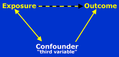
Multiple logistic regression is used to explore associations between one (dichotomous) outcome variable and two or more exposure variables (which may be continuous, ordinal or categorical). The purpose of multiple logistic regression is to isolate the relationship between the exposure variable and the outcome variable from the effects of one or more other variables (called covariates or confounders). For example, you can answer questions like, "How does calcium supplement use affect the probability of receiving treatment for osteoporosis, after accounting for (or unconfounded by, or independent of, or holding constant) age, income, etc.?" This process of accounting for covariates or confounders is called adjustment. For example, say that the prevalence of osteoporosis treatment tends to be lower in younger people; and younger people are less likely to take calcium supplements. In this case, inferences about osteoporosis treatment and calcium supplement use get confused by the effect of age on supplement use and osteoporosis treatment. This kind of "confusion" is called confounding (and these covariates are sometimes called confounders). Confounders are variables which are associated with both the exposure and outcome of interest. This relationship is shown in the following figure.
Diagram of the Relationship between Exposure, Outcome, and the Confounder

You can use multiple logistic regression to adjust for confounding and isolate the relationship of interest. The process of accounting for covariates is also called adjustment.
Comparing the results of simple and multiple logistic regression can help to answer the question, "How much did the covariates in the model alter the relationship between exposure and outcome (i.e., How much confounding was there)?"
Research Question
In this module, you will assess the association between calcium supplement use (the exposure variable) and the likelihood of receiving treatment for osteoporosis (the outcome). You will look at both simple logistic regression and then multiple logistic regression. The multiple logistic regression model will include age, race/ethnicity, and body mass index (BMI) as covariates. This analysis will answer the question, “What is the effect of calcium supplement use on the likelihood of receiving treatment for osteoporosis – after controlling for age, race/ethnicity, and body mass index (BMI)?”
Dependent Variable and Independent Variables
As noted, the dependent variable Y for a Logistic Regression is dichotomous, which means that it can take on one of two possible values. NHANES includes many questions where people must answer either “yes” or “no”; these include questions like “Has the doctor ever told you that you have congestive heart failure?”. Alternatively, you can create dichotomous variables by setting a threshold (e.g., “diabetes” = 1 if fasting blood sugar > 126 and “diabetes”=0 otherwise); or by combining information from several variables. In this module, we will use a dichotomous variable called “treatosteo” indicating osteoporosis treatment. In SUDAAN, and SAS Survey Procedures the dependent variable is coded as 1 (for having the outcome) and 0 (for not having the outcome). A participant was coded as having had treatment for osteoporosis if he or she responded “yes” to OSQ.070 (“{Were you/Was SP} treated for osteoporosis?”) from the osteoporosis questionnaire, and was set to “no” if he or she responded “no” to OSQ.070 or to OSQ.060 (“Has a doctor ever told {you/SP} that {you/s/he} had osteoporosis, sometimes called thin or brittle bones?”) from the osteoporosis questionnaire. (The SAS code to create this variable is found in the “Supplement Program” sample SAS code.) In this example, for people who receive treatment for osteoporosis, the treatosteo variable would have a value of 1, while the variable would have a value of 0 for people who were are not receiving treatment.
In logistic regression, the independent variables Xj can be categorical (e.g., gender, race), ordinal (e.g., supplement use (y/n), age groups, BMI categories), or continuous (e.g., continuous BMI). There are different ways that one can define categorical variables using indicator, or “dummy” variables. One common way is to define a reference category, i.e., the category to which the other levels of the categorical variable are compared.
Note that getting statistical packages like SUDAAN and SAS Survey to run analyses is the easy part of regression. What is not easy is knowing which variables to include in your analyses, how to represent them, and when to worry about confounding; determining if your models are any good; and knowing how to interpret them. These tasks require thought, training, experience, and respect for the underlying assumptions of regression. Remember, garbage in - garbage out.
Finally, remember that NHANES analyses can only establish associations and not causal relationships. This is because the data are cross-sectional, so there is no way to establish temporal sequences (i.e., which came first the "exposure" or the "outcome"?).
Logit Function
Because you are trying to find associations between risk factors and a condition, you need a formula that will allow you to link these variables. The logit function that is used in logistic regression is also known as the link function because it connects, or links, the values of the independent variables to the probability of occurrence of the event defined by the dependent variable.
Logit Model

In the logit formula above, Pr(Y=1) means the “probability that Y=1”, or the probability that the event occurs. In this equation ‘log' indicates natural log.
Optional: Learn more about odds ratios, linear and logistic regression
Conceptually, linear and logistic regression are very similar: you are trying to show the relationship between some exposures and an outcome. So why is the logit formula, with the log term, so fearsome?
The difference is in the nature of the outcome variable. It is continuous in linear regression, but dichotomous in logistic regression, and that creates a problem.
Imagine you wanted to see how supplement intake (a continuous variable) relates to age (a continuous variable). The output of linear regression, the b coefficient, a number anywhere from - ∞ to + ∞ , estimates how much a person’s supplement intake differs with every 1 year change in age.
Now you want to see how the chance, or probability, of taking supplements (yes/no, a dichotomous variable) relates to age. The linear regression approach won’t work if the outcome variable is a probability. That is because probabilities only range from 0 (i.e., no chance) to 1 (i.e. certain), but, as noted, the b coefficients could be negative (i.e. even less than "no chance") or greater than 1 (i.e., greater than "certain").
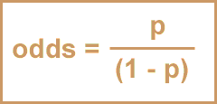
Logistic regression is a really clever way around this problem. It works by transforming probabilities to odds. “Odds” are a ratio,

where p is the probability that X happens and (1-p) is the probability that X does not happen.
Transforming to odds takes care of the “negative number” problem since, as is clear from the formula, odds range from 0 to infinity. Now comes the cleverest part: the odds are then further transformed into log form:

Why? Because log odds range from - ∞ to + ∞; that means the results of the logistic regression equation (i.e., the beta coefficient) can be interpreted just like those of linear regression: how much does the likelihood of the outcome change with a 1 unit change in the exposure. But here, “likelihood” is not a probability, but the log odds. Consider the relationship between supplement use and gender. If the chance of reporting supplement use is p, then:
The log odds of supplement use if you are a male

The log odds of supplement use if you are a female

The effect of gender then is just the difference:

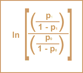
As you may remember, the difference of logs is the same as the log of their ratio, so:

The output of a logistic regression analysis the ß coefficient would show the relationship between supplement use and gender as follows:

Pay attention to the ratio: its the log of the ratio of odds. A ratio of odds is (reasonably enough) called an odds ratio. So the beta coefficient is actually the log odds ratio, which is easily transformed into a regular odds ratio, the usual output of logistic regression:

Bottom line: Logistic regression analysis tells you how much an increment in a given exposure variable affects the odds of the outcome.
Click to hide optional content
Output of Logistic Regression
The statistics of primary interest in logistic regression are the beta coefficients (ß1,ß2, ß3...), their standard errors, and their p-values. Like other statistics, the standard errors are used to calculate confidence intervals around the beta coefficients.
It is easy to transform the beta coefficients into a more interpretable format, the odds ratio, as follows:
eß= odds ratio.
If Xj is a dichotomous variable with values of 1 or 0, then the beta coefficient represents the log odds that an individual will have the event for a person with Xj=1 versus a person with Xj=0. In a multivariate model, this beta coefficient is the independent effect of variable Xj on Yi after adjusting for all other covariates in the model. The odds ratio eß represents the odds that an individual will have the event for a person with Xj= 1 versus an individual with Xj=0.
If Xj is a continuous variable, then the eß represents the odds that an individual will have the event for a person with Xj=m+1 versus an individual with Xj=m. In other words, for every one unit increase in Xj, the odds of having the event Yi changes by eß adjusting for all other covariates in a multivariate model.
A summary table about interpretation of beta coefficients is provided below:
| Independent Variable Type | Example Variables | The beta coefficient in simple logistic regression | The beta coefficient in multiple logistic regression |
|---|---|---|---|
| Continuous | height, weight, LDL |
The change in the log odds of the dependent variable per 1 unit change in the independent variable. |
The change in the log odds of dependent variable per 1 unit change in the independent variable after controlling for the confounding effects of the covariates in the model. |
| Categorical (also known as discrete) | Supplement use (two subgroups – yes and no. This example will use no as the reference group.) |
The difference in the log odds of the dependent variable for one value of the categorical variable vs. the reference group (for example, between supplement users, and the reference group, non-users). |
The difference in the log odds of the dependent variable for one value of the categorical variable vs. the reference group (for example, between supplement users, and the reference group, non-users), after controlling for the confounding effects of the covariates in the model. |
Odds and odds ratios are not the same as risk and relative risks.
In particular, odds and probability are two different ways to express the likelihood of an outcome.
Here are their definitions and some examples.
Table of Differences between Odds and Probability
| Definition | Example: Getting heads in 1 flip of a coin | Example: Getting a 1 in a single roll of a die | |
|---|---|---|---|
| Odds | # of times something |
= 1/1 = 1 (or 1:1) |
= 1/5 = 0.2 (or 1:5) |
| Probability | # of times something |
= 1/2 = .5 (or 50%) |
= 1/6 = .16 (or 16%) |
The above example illustrates the difference between odds and probabilities. In the example, the odds of getting a 1 in a single roll of a die is 20%, whereas the probability is 16%. The same is true for odds ratios and relative risk. Both are ratios of the odds or probability of the event for one group compared to another. For example, if we wanted to know the odds ratio of rolling a 1 with a blue die compared to a red die.
Few people think in terms of odds. Many people equate odds with probability and thus equate odds ratios with risk ratios. When the outcome of interest is uncommon (i.e., it occurs less than 10% of the time), such confusion makes little difference, since odds ratios and risk ratios are approximately equal. When the outcome is more common, however, the odds ratio increasingly overstates the risk ratio. So, to avoid confusion, when event rates are high, odds ratios should be converted to risk ratios. (Schwartz LM, Woloshin S, Welch HG. Misunderstandings about the effects of race and sex on physicians’ referrals for cardiac catheterization. N Engl J Med 1999;341:279–83) There are simple methods of conversion for both crude and adjusted data. (Zhang J, Yu KF. What's the relative risk? A method of correcting the odds ratio in cohort studies of common outcomes. JAMA 1998;280:1690-1691. Davies HT, Crombie IK, Tavakoli M. When can odds ratios mislead? BMJ 1998;316:989-991)
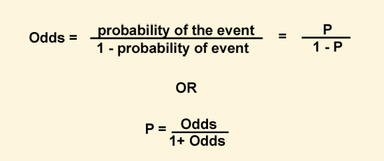
The following formulas demonstrate how to convert between probability and odds.

![]() Close Window
to return to module page.
Close Window
to return to module page.