Task 2: Key Concepts about Understanding Measurement Error

Types of Measurement Error

Statisticians understand that every survey measurement is an estimate of the true value of the thing being measured—whether it is dietary intake, physical activity, or some physiologic indicator such as blood pressure.  They call the difference between the measurement and the true value “measurement error,” but in this context, “error” does not mean “mistake.”  Rather, measurement error is understood to be an inherent part of data collection and analysis.  Nonetheless, because truth is the ideal, survey researchers attempt to minimize measurement error when collecting data, and statisticians adjust for existing error to minimize its effects.

Measurement error can be either random (non-systematic) or biased (systematic).  Random error is non-systematic because it contributes variability but does not influence the sample average.  Bias, on the other hand, occurs when measurements consistently depart in the same direction from the true value. 

 

Figure 1. Examples of bias and/or error

 

 

 

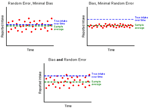
All sampled data contain random errors; some of these are positive and some are negative, but they balance out.  For example, individuals do not consume exactly the same amount of energy every day; yet, there is some true usual amount of energy that they consume over time.  If we could obtain perfectly recalled 24-hour dietary data from survey participants, we would assume that each recall measures the individual’s usual intake with some random error—i.e., that some recalls will be greater than usual and others less than usual, but that on average they approximate the true usual intake. Unfortunately, however, the inaccuracies inherent in self-reported intakes are not purely random, and thus, bias is introduced. 

Bias is potentially more serious than random error because it affects the mean of the sample, and can result in incorrect conclusions and estimates.  The same degree of bias may occur across all individuals in a sample, or differential bias can be associated with a particular characteristic.  For example, there is a general tendency across the population to under-report dietary intake, on both recalls and food frequency questionnaires.  This tendency varies by body weight status of the individual, such that overweight individuals under-report to a greater degree than do normal weight persons (the small percentage of the population that is underweight actually has a tendency to over-report their intakes).

 

Examples of Measurement Error in Dietary Data

The table below shows examples of random error and bias that can be found in each of the major types of dietary data.

Examples of Measurement Error in Dietary Data

Dietary Data Type	Random Error	Bias
Dietary Recall Data	Individuals tend to eat more on some days than others, so some 24-hour recalls will reflect greater-than-usual intakes while others will reflect less-than-usual amounts Standard nutrient values associated with foods in the database may be somewhat higher or lower than actual amounts of nutrients consumed	Generalized bias toward under-reporting of total energy May be differential under-reporting of some foods and nutrients and not others; not much is known about this
Food Frequency Questionnaire Data	Difficulties with cognition and recall lead to inaccurate and imprecise reporting	Generalized bias toward under-reporting of total energy May be differential under-reporting of some foods and nutrients and not others; not much is known about this
Dietary Supplement Data	Slight variations in the nutrient content of supplements from dose to dose Reporting errors	Differences between actual dietary supplement formulations and what the database states

 

Implications of Measurement Error in Dietary Data

Measurement error in dietary data has several practical implications.  Measurement error can seriously attenuate the relationship between dietary data and other factors, such as a health outcome.  That is, the analyses would be less likely to indicate a relationship between diet and disease even if one truly existed. 

Moreover, as shown in Figure 2 below, the relatively large within-person variation (among the days) in 24-hour recall data, if left unadjusted, leads to distributions of intake that are wider (red curve below) than distributions of true usual intake (blue curve below).  Because the single-day distribution includes unusual days—such as days of feasting and days of fasting—the red curve stretches further in each direction, causing it to be flatter and wider than the distribution of true usual (long-run average) intakes. 

Finally, the tendency toward underreporting, at least in energy intakes, indicates that reported intakes are also generally less than true intakes.  This underreporting is demonstrated by the fact that the blue curve is to the right of the red curve.

Figure 2. Relationship between reported intake, estimated usual intake, and true usual intake*

 

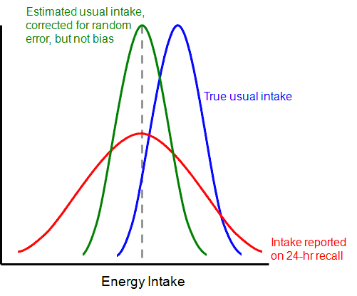
*Note: This is a conceptual drawing, not a depiction of real data.

 

Some of these problems have been addressed with statistical methods of adjustment.  Measurement error models can be used to analyze diet-disease relationships, and methods have been developed to estimate usual intakes that adjust for the problems associated with large within-person variation.  Unfortunately, no standard adjustment currently exists for correcting for underreporting bias.  Therefore, these models and methods require an assumption that 24-hour recalls are unbiased for usual intake, in spite of biomarker-based evidence to the contrary.  Nonetheless, these are the best methods available and represent state-of-the-art practice.  For this reason, it is important to acknowledge these caveats when reporting analyses. 

The green curve in the figure above shows an estimated distribution of intake corrected for within-individual variability (random error) but not for underreporting (bias).  Note that the means of the green and red curves are the same, even though the overall shapes are different.  The sample analyses in this course capitalize on this fact, in that unadjusted means of the reported intakes are interpreted as the means of the population distribution of usual intake. More sophisticated techniques are needed to estimate the entire distribution of usual intake, rather than just its mean.