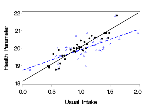
When interest is on relating usual intake of a dietary constituent to disease or a biomarker (termed “health parameters” in this module), we must consider the impact of measurement error in dietary assessment on the estimate of the relationship of interest. Random dietary measurement error will lead to an attenuated (weakened) estimate of the true relationship and a loss of statistical power. To get an (almost) unbiased estimate of the true relationship we can use an approach called regression calibration.
Figure 1. The effects of random error on the relationship between usual intake and a health parameter. The black dots and solid regression line represent the true relationship, and the blue triangles and dashed line represent the observed attenuated relationship.

Statistically, we can represent the relationship between the health outcome O and true usual intake T as
O = a 0 + a 1 T + e
Where α0 is the intercept, α1 is the slope of the regression of O on T, andε is error. For simplicity, we are representing the relationship between O and T as linear. In fact, the health parameter may be continuous or categorical. For example, when modeling a disease outcome, logistic regression might be used. In this statistical model,α1 is the parameter of most interest, as it represents the relationship between true usual intake and the health parameter. Unfortunately, we do not have a measure of T, so it cannot be estimated directly. Instead of T, we have R, our 24-hour recall data that are measured with error:
![]()
The tildes represent that the relationships that are estimated with the data measured with error differ from those that we would have observed if we had a measure of true usual intake. By relating our imperfect measure R to truth T, we can quantify the difference between α1 and ![]() . First, we define:
. First, we define:
R = T + U
where U is the random error associated with R. The above relationship makes an important assumption – that R is measured with error, but that this error is random, i.e., R provides an unbiased estimate of T. This is the assumption we make throughout the tutorial for the 24-hour recall.
Next, we can use the definition of the slope, and the substitution of the formula above for R to show that:

where λ=var(T)/[var(T) + var(U)]. We assume that T and U are independent and that the measurement error is non-differential with respect to the outcome. This factor, λ, is termed the attenuation factor, and it is the slope of the regression of T on R. In the case of logistic regression, the relationship between the true relative risk (RRT) and the relative risk observed when R is used rather than T (RRR), are associated by the formula:
![]()
The attenuation factor also is related to the correlation between truth T and the reported value R through:

When attenuation occurs, there is a loss of power for testing that the slope is significantly different from 0 (i.e., no relationship). This power is directly related to the inverse of the square of the correlation between T and R, i.e., the sample size required to detect an effect using R is ![]() times the sample size required if T were available.
times the sample size required if T were available.
To get an (almost) unbiased estimate of α1 we can use an approach called regression calibration. In regression calibration, instead of using R for T in the disease model we use the expected value of T, given that we know R:
![]()
Intuitively, this estimator is our best estimate of T, given what we do know from the 24-hour recall data. This value is the Empirical Bayes estimator (or best linear unbiased predictor) for the linear mixed model, when no transformation of the data is necessary. Unfortunately, transformation is usually required and numerical integration needs to be used. This may be done using the NCI method.
If we have covariates X in our health parameter model, which we almost always do, i.e.,
![]()
then we also must include X in our regression calibration predictor,![]() In addition, even if X is not in the health model, then we can still use it to obtain
In addition, even if X is not in the health model, then we can still use it to obtain ![]() . This gives us a better estimate of T, and, consequently, a better estimate of α1 . This is called extended regression calibration. These covariates should not be related to the health parameter given truth, however.
. This gives us a better estimate of T, and, consequently, a better estimate of α1 . This is called extended regression calibration. These covariates should not be related to the health parameter given truth, however.
In the health model, a transformation of T, rather than T on the original scale, may provide a better model fit. Therefore, this method uses a Box-Cox transformation of T in the health model.
It is important to note that regression calibration does not restore power; it is used to obtain an estimate of the true parameter relating diet to the health outcome (e.g., relative risk).
![]() Close Window
to return to module page.
Close Window
to return to module page.