Work loop
The work loop technique is used in muscle physiology to evaluate the mechanical work and power output of skeletal or cardiac muscle contractions via in vitro muscle testing of whole muscles, fiber bundles or single muscle fibers. This technique is primarily used for cyclical contractions such as the rhythmic flapping of bird wings[1] or the beating of heart ventricular muscle.[2]
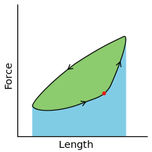
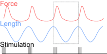
To simulate the rhythmic shortening and lengthening of a muscle (e.g. while moving a limb), a servo motor oscillates the muscle at a given frequency and range of motion observed in natural behavior. Simultaneously, a burst of electrical pulses is applied to the muscle at the beginning of each shortening-lengthening cycle to stimulate the muscle to produce force. Since force and length return to their initial values at the end of each cycle, a plot of force vs. length yields a 'work loop'. Intuitively, the area enclosed by the loop represents the net mechanical work performed by the muscle during a single cycle.
History
Classical studies from the 1920s through the 1960s characterized the fundamental properties of muscle activation (via action potentials from motor neurons), force development, length change and shortening velocity.[3] However, each of these parameters were measured while holding other ones constant, making their interactions unclear. For instance, force-velocity and force-length relationships were determined at constant velocities and loads. Yet during locomotion, neither muscle velocity nor muscle force are constant. In running, for example, muscles in each leg experience time-varying forces and time-varying shortening velocities as the leg decelerates and accelerates from heelstrike to toeoff. In such cases, classical force-length (constant velocity) or force-velocity (constant length) experiments might not be sufficient to fully explain muscle function.[4]
In 1960, the work loop method was introduced to explore muscle contractions of both variable speed and variable force. These early work loop experiments characterized the mechanical behavior of asynchronous muscle (a type of insect flight muscle).[5] However, due to the specialized nature of asynchronous muscle, the work loop method was only applicable for insect muscle experiments. In 1985, Robert K. Josephson modernized the technique to evaluate properties of synchronous muscles powering katydid flight[6] by stimulating the muscle at regular time intervals during each shortening-lengthening cycle. Josephson's innovation generalized the work loop technique for wide use among both invertebrate and vertebrate muscle types, profoundly advancing the fields of muscle physiology and comparative biomechanics.
Work loop experiments also allowed greater appreciation for the role of activation & relaxing kinetics in muscle power and work output. For instance, if a muscle turns on and off more slowly, the shortening and lengthening curves will be shallower and closer together, resulting in decreased work output. "Negative" work loops were also discovered, showing that muscle lengthening at higher force than the shortening curve can result in net energy absorption by the muscle, as in the case of deceleration or constant-speed downhill walking.
In 1992, the work loop approach was extended further by the novel use of bone strain measurements to obtain in vivo force. Combined either with estimates of muscle length changes or with direct methods (e.g. sonomicrometry), in vivo force technology enabled the first in vivo work loop measurements.[7]
Work loop analysis
Positive, negative and net work
A work loop combines two separate plots: force vs. time and length vs. time. When force is plotted against length, a work loop plot is created: each point along the loop corresponds to a force and a length value at a unique point in time. As time progresses, the plotted points trace the shape of the work loop. The direction in which the work loop is traced through time is a critical feature of the work loop. As the muscle shortens while generating a tensile force (i.e. "pulling"), then, by convention in, the muscle is said to be performing positive work during that phase. As the muscle lengthens (while still generating a tensile force), the muscle is performing negative work (or, alternatively, that positive work is being performed on the muscle). Thus a muscle generating force while shortening is said to output 'positive work' (i.e. generating work), whereas a muscle generating force while lengthening produces 'negative work' (i.e. absorbing work). Over an entire cycle, there is typically some positive, and some negative work; if the overall cycle is counter-clockwise vs. clockwise work loop represents overall work generation vs. work absorption, respectively.[8] For example during a jump, the leg muscles generate work to increase the body's speed away from the ground, yielding counter-clockwise work loops. When landing, however, the same muscles absorb work to decrease the body's speed, yielding clockwise work loops. Furthermore, a muscle can produce positive work followed by negative work (or vice versa) within a shortening-lengthening cycle, causing a 'figure 8' work loop shape containing both clockwise and counter-clockwise segments.[9]
Since work is defined as force multiplied by displacement, the area of the graph shows the mechanical work output of the muscle. In a typical work-generating instance, the muscle shows a rapid curvilinear rise in force as it shortens, followed by a slower decline during or shortly before the muscle begins the lengthening phase of the cycle. The area beneath the shortening curve (upper curve) gives the total work done by the shortening muscle, while the area beneath the lengthening curve (lower curve) represents the work absorbed by the muscle and turned into heat (done by either environmental forces or antagonistic muscles). Subtracting the latter from the former gives the net mechanical work output of the muscle cycle, and dividing that by the cycle duration gives net mechanical power output.[10]
Inferring muscle function from work loop shape
Hypothetically, a square work loop (area = max force x max displacement) would represent the maximum work output of a muscle operating within a given force and length range.[11][12] Conversely, a flat line (area = 0) would represent the minimum work output. For example, a muscle that generates force without changing length (isometric contraction) will show a vertical line 'work loop'. Reciprocally, a muscle that shortens without changing force (isotonic contraction) will show a horizontal line 'work loop'. Finally, a muscle can behave like a spring which extends linearly as a force is applied. This final case would yield a slanted straight line 'work loop' where the line slope is the spring stiffness.[13]
Work loop experimental approach
Work loop experiments are most often performed on muscle tissue isolated either from invertebrates (e.g. insects[14] and crustaceans[15]) or small vertebrates (e.g. fish,[16] frogs,[17] rodents[18]). The experimental technique described below applies both to in vitro and in situ approaches.
Experimental setup
Following humane procedures approved by IACUC, the muscle is isolated from the animal (or prepared in situ), attached to the muscle testing apparatus and bathed in oxygenated Ringer's solution or Krebs-Henseleit solution maintained at a constant temperature. While the isolated muscle is still living, the experimenter then applies two manipulations to test muscle function: 1) Electrical stimulation to mimic the action of a motor neuron and 2) strain (muscle length change) to mimic the rhythmic motion of a limb. To elicit muscle contraction, the muscle is stimulated by a series of electrical pulses delivered by an electrode to stimulate either the motor nerve or the muscle tissue itself. Simultaneously, a computer-controlled servo motor in the testing apparatus oscillates the muscle while measuring the force generated by the stimulated muscle. The following parameters are modulated by the experimenter to influence muscle force, work and power output:
- Stimulation duration: The time period over which the muscle receives electrical stimulation
- Stimulation pulse frequency: The number of stimulation pulses per stimulation duration
- Stimulation phase: The time delay between the onset of stimulation and muscle length change
- Strain amplitude: The difference between the maximum and minimum values of the length oscillation pattern
- Strain/cycle frequency: The number of shortening-lengthening periods per time period
Calculating muscular work and power from experimental data
Calculation of either muscle work or power requires collection of muscle force and length (or velocity) data at a known sampling rate. Net work is typically calculated either from instantaneous power (muscle force x muscle velocity) or from the area enclosed by the work loop on a force vs. length plot. Both methods are mathematically equivalent and highly accurate, however the 'area inside the loop' method (despite its simplicity) can be tedious to carry out for large data sets.
Method 1: Instantaneous power method
Step 1) Obtain muscle velocity by numerical differentiation of muscle length data. Step 2) Obtain instantaneous muscle power by multiplying muscle force data by muscle velocity data for each time sample. Step 3) Obtain net work (a single number) by numerical integration of muscle power data. Step 4) Obtain net power (a single number) by dividing net work by the time duration of the cycle.
Method 2: Area inside the loop method
The area inside the work loop can be quantified either 1) digitally by importing a work loop image into ImageJ, tracing the work loop shape and quantifying its area. Or, 2) manually by printing a hard copy of the work loop graph, cutting the inner area and weighing it on an analytical balance. Net work is then divided by the time duration of the cycle to obtain net power.
Applications to skeletal muscle physiology
A significant advantage of the work loop technique over assessments of skeletal muscle power in humans is that confounding factors associated with skeletal muscle function masks true power production at the skeletal muscle level. The most notable confounding factors include the influence of the central nervous system limiting the ability to generate maximal power output, examinations of whole muscle groups rather than individual skeletal muscles, bodily inertia, and motivational aspects associated with sustained muscle activity. Additionally, measures of muscle fatigue are not affected by fatigue of the central nervous system. By adopting the work loop technique in an isolated muscle model, these confounding factors are eliminated, thus allowing for a closer examination of the muscle-specific changes in work loop power output in response to a stimulus. Moreover, usage of the work loop technique as opposed to other modes of contraction, such as isometric, isotonic and isovelocity, allows for a better representation of the changes in mechanical work of the skeletal muscle in response to an independent variable, such as the direct application of caffeine,[21][22][23][24][25] sodium bicarbonate,[26] and taurine[27] to an isolated skeletal muscle, and the changes in work loop power output and fatigue resistance during ageing[28][29][30] and in response to an obesogenic diet.[31][32]
Applications to animal locomotion
Identifying muscle functional roles: motors, brakes, springs, or struts
As a “motor” the muscle does work on the environment resulting in positive work in the work loop in the counter-clockwise direction. When positive work happens the length of the muscle will increase followed by an increase in force before reaching a peak. When the peak is reached the muscle will shorten along with a decrease in force.[33] An example of positive work being done in the environment would be scallops swimming.[34]
As a “brake” the muscle is able to absorb energy from the environment.[35] This then results in negative work in the work loop in a clockwise direction. The result is a shortening of the muscles as well as a decrease in force output. After the muscle is done absorbing the energy from the environment, the length of the muscle then returns to normal with increased force. In cockroaches, there are legs that act purely as “brakes” to stop the animal’s movement.
As a “spring” the muscles are able to alter between states of motion, thus producing negative work [36][37] this negative work results from the movement and changing of the muscles position in bird flight and human legs in order to produce more energy. The “springs” in these muscles absorb the energy from the environment and redirect it, then outputting that absorbed energy to make repeated movements more energy efficient.
As a “strut” the muscle can output a force and then hold the muscle length. In fish movement the body moves back and forth to produce work but as the fish moves the muscles move the energy down the length of the fish. As the energy passes the muscle the muscle then holds as a “strut”. The length of the muscle as a “strut” remains constant.[38]
Asymmetrical muscle length trajectories
Originally, workloops imposed a sinusoidal length change on the muscle, with equal time lengthening and shortening. However, in vivo muscle length change often has greater than half the cycle shortening, and less than half lengthening. Imposing these "asymmetrical" stretch-shorten cycles can result in higher work and power outputs, as shown in treefrog calling muscles.[39]
Applications to cardiac muscle physiology
References
- http://jeb.biologists.org/content/204/21/3587.full
- http://jeb.biologists.org/content/201/19/2723.full.pdf
- Hill, A. V. (1970). First and last experiments in muscle mechanics. London: Cambridge University Press.
- http://jeb.biologists.org/content/202/23/3377.short
- http://rspb.royalsocietypublishing.org/content/152/948/311
- http://jeb.biologists.org/cgi/content/abstract/114/1/493
- http://jeb.biologists.org/content/164/1/1.abstract?sid=106f650c-81c1-4d4e-9cac-4e10039f7131
- Biewener, A. (2003). Animal Locomotion. Oxford: Oxford University Press.
- http://jp.physoc.org/content/549/3/877.short
- Biewener, A. (2003). Animal Locomotion. Oxford: Oxford University Press.
- Biewener, A. (2003). Animal Locomotion. Oxford: Oxford University Press.
- http://jeb.biologists.org/content/206/8/1363
- Wainwright, S. A. (1982). Mechanical design in organisms: Princeton Univ Pr.
- http://jeb.biologists.org/cgi/content/abstract/114/1/493
- http://jeb.biologists.org/content/145/1/45
- http://jeb.biologists.org/content/151/1/453.abstract?sid=b67053d6-9126-41c8-afb4-bc797b62a4bc
- http://jp.physoc.org/content/549/3/877
- http://jeb.biologists.org/content/200/24/3119.abstract?sid=b6d72d95-cd9d-4378-9294-02f9973ad04a
- http://jeb.biologists.org/content/151/1/453
- http://jp.physoc.org/content/549/3/877.short
- https://bpspubs.onlinelibrary.wiley.com/journal/14765381
- Tallis, Jason; James, Rob S.; Cox, Val M.; Duncan, Michael J. (2012). "The effect of physiological concentrations of caffeine on the power output of maximally and submaximally stimulated mouse EDL (fast) and soleus (slow) muscle". Journal of Applied Physiology. 112 (1): 64–71. doi:10.1152/japplphysiol.00801.2011. PMID 21979804.
- Tallis, Jason; James, R. S.; Cox, V. M.; Duncan, M. J. (2017). "Is the ergogenicity of caffeine affected by increasing age? The direct effect of a physiological concentration of caffeine on the power output of maximally stimulated edl and diaphragm muscle isolated from the mouse". The Journal of Nutrition, Health & Aging. 21 (4): 440–448. doi:10.1007/s12603-016-0832-9. PMID 28346571.
- James, Rob. S.; Wilson, Robbie S.; Askew, Graham N. (2004). "Effects of caffeine on mouse skeletal muscle power output during recovery from fatigue". Journal of Applied Physiology. 96 (2): 545–552. doi:10.1152/japplphysiol.00696.2003. PMID 14506097.
- James, Rob S.; Kohlsdorf, Tiana; Cox, Val M.; Navas, Carlos A. (2005). "70 μM caffeine treatment enhances in vitro force and power output during cyclic activities in mouse extensor digitorum longus muscle". European Journal of Applied Physiology. 95 (1): 74–82. doi:10.1007/s00421-005-1396-2. PMID 15959797.
- Higgins, M. F.; Tallis, J.; Price, M. J.; James, R. S. (2013). "The effects of elevated levels of sodium bicarbonate (NaHCO3) on the acute power output and time to fatigue of maximally stimulated mouse soleus and EDL muscles". European Journal of Applied Physiology. 113 (5): 1331–1341. doi:10.1007/s00421-012-2557-8. PMID 23203385.
- Tallis, Jason; Higgins, Matthew F.; Cox, Val. M.; Duncan, Michael J.; James, Rob. S. (2014). "Does a physiological concentration of taurine increase acute muscle power output, time to fatigue, and recovery in isolated mouse soleus (slow) muscle with or without the presence of caffeine?". Canadian Journal of Physiology and Pharmacology (Submitted manuscript). 92 (1): 42–49. doi:10.1139/cjpp-2013-0195. hdl:10545/621162. PMID 24383872.
- Tallis, Jason; James, Rob S.; Little, Alexander G.; Cox, Val M.; Duncan, Michael J.; Seebacher, Frank (2014). "Early effects of ageing on the mechanical performance of isolated locomotory (EDL) and respiratory (diaphragm) skeletal muscle using the work-loop technique". American Journal of Physiology. Regulatory, Integrative and Comparative Physiology. 307 (6): R670–R684. doi:10.1152/ajpregu.00115.2014. PMID 24990861.
- Tallis, Jason; Higgins, Matthew F.; Seebacher, Frank; Cox, Val M.; Duncan, Michael J.; James, Rob S. (2017). "The effects of 8 weeks voluntary wheel running on the contractile performance of isolated locomotory (soleus) and respiratory (diaphragm) skeletal muscle during early ageing". The Journal of Experimental Biology. 220 (20): 3733–3741. doi:10.1242/jeb.166603. PMID 28819051.
- Hill, Cameron; James, Rob S.; Cox, Val M.; Tallis, Jason (2018). "The Effect of Increasing Age on the Concentric and Eccentric Contractile Properties of Isolated Mouse Soleus and Extensor Digitorum Longus Muscles". The Journals of Gerontology: Series A. 73 (5): 579–587. doi:10.1093/gerona/glx243. PMID 29236945.
- Tallis, Jason; Hill, Cameron; James, Rob S.; Cox, Val M.; Seebacher, Frank (2017). "The effect of obesity on the contractile performance of isolated mouse soleus, EDL, and diaphragm muscles". Journal of Applied Physiology. 122 (1): 170–181. doi:10.1152/japplphysiol.00836.2016. PMID 27856719.
- Seebacher, F.; Tallis, J.; McShea, K.; James, R. S. (2017). "Obesity-induced decreases in muscle performance are not reversed by weight loss". International Journal of Obesity. 41 (8): 1271–1278. doi:10.1038/ijo.2017.81. PMID 28337027.
- A. A. Biewener, W. R. Corning, B. T. Tobalske, J. Exp.Biol. 201, 3293 (1998).
- Michael H. Dickinson, Claire T. Farley, Robert J. Full, M. A. R. Koehl, Rodger Kram, and Steven Lehman.Science 7 April 2000: 288 (5463), 100-106.
- R. J. Full, D. R. Stokes, A. N. Ahn, R. K. Josephson, J.Exp. Biol. 201, 997 (1998).
- M. S. Tu and M. H. Dickinson, J. Exp. Biol. 192, 207(1994).
- M. H. Dickinson and M. S. Tu, Comp. Biochem.Physiol. A 116, 223 (1997)
- R. E. Shadwick, J. F. Steffenson, S. L. Katz, T. Knower, Am. Zool. 38, 755 (1998)
- http://jeb.biologists.org/cgi/content/abstract/202/22/3225