Pulsatile flow

In fluid dynamics, a flow with periodic variations is known as pulsatile flow, or as Womersley flow. The flow profiles was first derived by John R. Womersley (1907–1958) in his work with blood flow in arteries.[1] The cardiovascular system of chordate animals is a very good example where pulsatile flow is found, but pulsatile flow is also observed in engines and hydraulic systems, as a result of rotating mechanisms pumping the fluid.

Equation

Four pulsatile flow profiles in a straight tube are shown. The first graph (in blue) shows the pressure gradient as a cosine function, and the other graphs (in red) show dimensionless velocity profiles for different Womersley numbers.

The pulsatile flow profile is given in a straight pipe by

u(r,t)=Re\left\{\sum _{n=0}^{N}{\frac {i\,P'_{n}}{\rho \,n\,\omega }}\left[1-{\frac {J_{0}(\alpha \,n^{1/2}\,i^{3/2}\,{\frac {r}{R}})}{J_{0}(\alpha \,n^{1/2}\,i^{3/2})}}\right]e^{in\omega t}\right\}\,,

where:

$u$	is the longitudinal flow velocity,
$r$	is the radial coordinate,
$t$	is time,
$α$	is the dimensionless Womersley number,
$ω$	is the angular frequency of the first harmonic of a Fourier series of an oscillatory pressure gradient,
$n$	are the natural numbers,
$P' n$	is the pressure gradient magnitude for the frequency $nω$ ,
$ρ$	is the fluid density,
$μ$	is the dynamic viscosity,
$R$	is the pipe radius,
$J 0 (\cdot)$	is the Bessel function of first kind and order zero,
$i$	is the imaginary number, and
$Re{\cdot$ }	is the real part of a complex number.

Properties

Womersley number

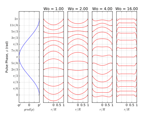
The pulsatile flow profile changes its shape depending on the Womersley number

\alpha =R\left({\frac {\omega \rho }{\mu }}\right)^{1/2}\,.

For $\alpha \lesssim 2$ , viscous forces dominate the flow, and the pulse is considered quasi-static with a parabolic profile. For $\alpha \gtrsim 2$ , the inertial forces are dominant in the central core, whereas viscous forces dominate near the boundary layer. Thus, the velocity profile gets flattened, and phase between the pressure and velocity waves gets shifted towards the core.

Function limits

Lower limit

The Bessel function at its lower limit becomes[2]

\lim _{z\to \infty }J_{0}(z)=1-{\frac {z^{2}}{4}}\,,

which converges to the Hagen-Poiseuille flow profile for steady flow for

\lim _{n\to 0}u(r,t)=-{\frac {P'_{0}}{4\mu }}\left(R^{2}-r^{2}\right)\,,

or to a quasi-static pulse with parabolic profile when

\lim _{\alpha \to 0}u(r,t)=Re\left\{-\sum _{n=0}^{N}{\frac {P'_{n}}{4\mu }}(R^{2}-r^{2})\,e^{in\omega t}\right\}=-\sum _{n=0}^{N}{\frac {P'_{n}}{4\mu }}(R^{2}-r^{2})\,\cos(n\omega t)\,.

In this case, the function is real, because the pressure and velocity waves are in phase.

Upper limit

The Bessel function at its upper limit it becomes[2]

\lim _{z\to \infty }J_{0}(z\,i)={\frac {e^{z}}{\sqrt {2\pi \,z}}}\,,

which converges to

\lim _{z\to \infty }u(r,t)=Re\left\{\sum _{n=0}^{N}{\frac {i\,P'_{n}}{\rho \,n\,\omega }}\left[1-e^{\alpha \,n^{1/2}\,i^{1/2}\left({\frac {r}{R}}-1\right)}\right]e^{in\omega t}\right\}=-\sum _{n=0}^{N}{\frac {\,P'_{n}}{\rho \,n\,\omega }}\left[1-e^{\alpha \,n^{1/2}\left({\frac {r}{R}}-1\right)}\right]\sin(n\,\omega \,t)\,.

This is highly reminiscent of the Stokes layer on an oscillating flat plate, or the skin-depth penetration of an alternating magnetic field into an electrical conductor. On the surface $u(r=R,t)=0$ , but the exponential term becomes negligible once $\alpha (1-r/R)$ becomes large, the velocity profile becomes almost constant and independent of the viscosity. Thus, the flow simply oscillates as a plug profile in time according to the pressure gradient,

\rho {\frac {\partial u}{\partial t}}=-\sum _{n=0}^{N}P'_{n}\,.

However, close to the walls, in a layer of thickness ${\mathcal {O}}(\alpha ^{-1})$ , the velocity adjusts rapidly to zero. Furthermore, the phase of the time oscillation varies quickly with position across the layer. The exponential decay of the higher frequencies is faster.

Derivation

For deriving the analytical solution of this non-stationary flow velocity profile, the following assumptions are taken:[3][4]

Fluid is homogeneous, incompressible and Newtonian;
Tube wall is rigid and circular;
Motion is laminar, axisymmetric and parallel to the tube's axis;
Boundary conditions are: axisymmetry at the centre, and no-slip condition on the wall;
Pressure gradient is a periodic function that drives the fluid;
Gravitation has no effect on the fluid.

Thus, the Navier-Stokes equation and the continuity equation are simplified as

\rho {\frac {\partial u}{\partial t}}=-{\frac {\partial p}{\partial x}}+\mu \left({\frac {\partial ^{2}u}{\partial r^{2}}}+{\frac {1}{r}}{\frac {\partial u}{\partial r}}\right)\,

and

{\frac {\partial u}{\partial x}}=0\,,

respectively. The pressure gradient driving the pulsatile flow is decomposed in Fourier series,

{\frac {\partial p}{\partial x}}(t)=\sum _{n=0}^{N}P'_{n}e^{in\omega t}\,,

where $i$ is the imaginary number, $\omega$ is the angular frequency of the first harmonic (i.e., $n=1$ ), and $P'_{n}$ are the amplitudes of each harmonic $n$ . Note that, $P'_{0}$ (standing for $n=0$ ) is the steady-state pressure gradient, whose sign is opposed to the steady-state velocity (i.e., a negative pressure gradient yields positive flow). Similarly, the velocity profile is also decomposed in Fourier series in phase with the pressure gradient, because the fluid is incompressible,

u(r,t)=\sum _{n=0}^{N}U_{n}e^{in\omega t}\,,

where $U_{n}$ are the amplitudes of each harmonic of the periodic function, and the steady component ( $n=0$ ) is simply Poiseuille flow

U_{0}=-{\frac {P'_{0}}{4\mu }}\left(R^{2}-r^{2}\right)\,.

Thus, the Navier-Stokes equation for each harmonic reads as

i\rho n\omega U_{n}=-P'_{n}+\mu \left({\frac {\partial ^{2}U_{n}}{\partial r^{2}}}+{\frac {1}{r}}{\frac {\partial U_{n}}{\partial r}}\right)\,.

With the boundary conditions satisfied, the general solution of this ordinary differential equation for the oscillatory part ( $n\geq 1$ ) is

U_{n}(r)=A_{n}\,J_{0}\left(\alpha \,{\frac {r}{R}}n^{1/2}\,i^{3/2}\right)+B_{n}\,Y_{0}\left(\alpha \,{\frac {r}{R}}n^{1/2}\,i^{3/2}\right)+{\frac {i\,P'_{n}}{\rho \,n\,\omega }}\,,

where $J_{0}(\cdot )$ is the Bessel function of first kind and order zero, $Y_{0}(\cdot )$ is the Bessel function of second kind and order zero, $A_{n}$ and $B_{n}$ are arbitrary constants, and $\alpha =R\surd (\omega \rho /\mu )$ is the dimensionless Womersley number. The axisymetic boundary condition ( $\partial U_{n}/\partial r|_{r=0}=0$ ) is applied to show that $B_{n}=0$ for the derivative of above equation to be valid, as the derivatives $J_{0}'$ and $Y_{0}'$ approach infinity. Next, the wall non-slip boundary condition ( $U_{n}(R)=0$ ) yields $A_{n}=-{\frac {i\,P'_{n}}{\rho \,n\,\omega }}{\frac {1}{J_{0}\left(\alpha \,n^{1/2}\,i^{3/2}\right)}}$ . Hence, the amplitudes of the velocity profile of the harmonic $n$ becomes

U_{n}(r)={\frac {i\,P'_{n}}{\rho \,n\,\omega }}\left[1-{\frac {J_{0}(\alpha \,n^{1/2}\,i^{3/2}\,{\frac {r}{R}})}{J_{0}(\alpha \,n^{1/2}\,i^{3/2})}}\right]={\frac {i\,P'_{n}}{\rho \,n\,\omega }}\left[1-{\frac {J_{0}(\Lambda _{n}\,{\frac {r}{R}})}{J_{0}(\Lambda _{n})}}\right]\,,

where $\Lambda _{n}=\alpha \,n^{1/2}\,i^{3/2}$ is used for simplification. The velocity profile itself is obtained by taking the real part of the complex function resulted from the summation of all harmonics of the pulse,

u(r,t)={\frac {P'_{0}}{4\mu }}\left(R^{2}-r^{2}\right)+Re\left\{\sum _{n=1}^{N}{\frac {i\,P'_{n}}{\rho \,n\,\omega }}\left[1-{\frac {J_{0}(\Lambda _{n}\,{\frac {r}{R}})}{J_{0}(\Lambda _{n})}}\right]e^{in\omega t}\right\}\,.

Flow rate

Flow rate is obtained by integrating the velocity field on the cross-section. Since,

{\frac {d}{dx}}\left[x^{p}J_{p}(a\,x)\right]=a\,x^{p}J_{p-1}(a\,x)\quad \Rightarrow \quad {\frac {d}{dx}}\left[x\,J_{1}(a\,x)\right]=a\,xJ_{0}(a\,x)\,,

then

Q(t)=\iint u(r,t)\,dA=Re\left\{\pi \,R^{2}\,\sum _{n=1}^{N}{\frac {i\,P'_{n}}{\rho \,n\,\omega }}\left[1-{\frac {2}{\Lambda _{n}}}{\frac {J_{1}(\Lambda _{n})}{J_{0}(\Lambda _{n})}}\right]e^{in\omega t}\right\}\,.

Velocity profile

Scaled velocity profiles of pulsatile flow are compared according to Womersley number.

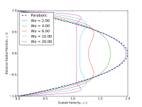
To compare the shape of the velocity profile, it can be assumed that

u(r,t)=f(r)\,{\frac {Q(t)}{A}}\,,

where

f(r)={\frac {u(r,t)}{\frac {Q(t)}{A}}}=Re\left\{\sum _{n=1}^{N}\left[{\frac {\Lambda _{n}\,J_{0}(\Lambda _{n})-\Lambda _{n}\,J_{0}(\Lambda _{n}\,{\frac {r}{R}})}{\Lambda _{n}\,J_{0}(\Lambda _{n})-2\,J_{1}(\Lambda _{n})}}\right]\right\}

is the shape function.[5] It is important to notice that this formulation ignores the inertial effects. The velocity profile approximates a parabolic profile or a plug profile, for low or high Womersley numbers, respectively.

Wall shear stress

For straight pipes, wall shear stress is

\tau _{w}=\mu \left.{\frac {\partial u}{\partial r}}\right|_{r=R}\,.

The derivative of a Bessel function is

{\frac {\partial }{\partial x}}\left[x^{-p}J_{-p}(a\,x)\right]=a\,x^{-p}J_{p+1}(a\,x)\quad \Rightarrow \quad {\frac {\partial }{\partial x}}\left[J_{0}(a\,x)\right]=-a\,J_{1}(a\,x)\,.

Hence,

\tau _{w}=Re\left\{\sum _{n=1}^{N}P'_{n}{\frac {R}{\Lambda _{n}}}{\frac {J_{1}(\Lambda _{n})}{J_{0}(\Lambda _{n})}}e^{in\omega t}\right\}\,.

Centre line velocity

If the pressure gradient $P'_{n}$ is not measured, it can still be obtained by measuring the velocity at the centre line. The measured velocity has only the real part of the full expression in the form of

{\tilde {u}}(t)=Re(u(0,t))\equiv \sum _{n=1}^{N}{\tilde {U}}_{n}\,\cos(n\,\omega \,t)\,.

Noting that $J_{0}(0)=1$ , the full physical expression becomes

u(0,t)=Re\left\{\sum _{n=1}^{N}{\frac {i\,P'_{n}}{\rho \,n\,\omega }}\left[{\frac {J_{0}(\Lambda _{n})-1}{J_{0}(\Lambda _{n})}}\right]e^{in\omega t}\right\}

at the centre line. The measured velocity is compared with the full expression by applying some properties of complex number. For any product of complex numbers ( $C=AB$ ), the amplitude and phase have the relations $|C|=|A||B|$ and $\phi _{C}=\phi _{A}+\phi _{B}$ , respectively. Hence,

{\tilde {U}}_{n}=\left|{\frac {i\,P'_{n}}{\rho \,n\,\omega }}\left[{\frac {J_{0}(\Lambda _{n})-1}{J_{0}(\Lambda _{n})}}\right]\right|\quad \Rightarrow \quad P'_{n}={\tilde {U}}_{n}\left|i\,\rho \,n\,\omega \left[{\frac {J_{0}(\Lambda _{n})}{1-J_{0}(\Lambda _{n})}}\right]\right|

and

{\tilde {\phi }}=0=\phi _{P'_{n}}+\phi _{U_{n}}\quad \Rightarrow \quad \phi _{P'_{n}}=\operatorname {phase} \left({\frac {i}{\rho \,n\,\omega }}\left[{\frac {1-J_{0}(\Lambda _{n})}{J_{0}(\Lambda _{n})}}\right]\right)\,,

which finally yield

{\frac {1}{\rho }}{\frac {\partial p}{\partial x}}=\sum _{n=1}^{N}{\tilde {U}}_{n}\left|i\,\rho \,n\,\omega \left[{\frac {J_{0}(\Lambda _{n})}{1-J_{0}(\Lambda _{n})}}\right]\right|\,\cos \left\{n\,\omega \,t+\operatorname {phase} \left({\frac {i}{\rho \,n\,\omega }}\left[{\frac {1-J_{0}(\Lambda _{n})}{J_{0}(\Lambda _{n})}}\right]\right)\right\}\,.

References

Womersley, J.R. (March 1955). "Method for the calculation of velocity, rate of flow and viscous drag in arteries when the pressure gradient is known". J. Physiol. 127 (3): 553–563. doi:10.1113/jphysiol.1955.sp005276. PMC 1365740. PMID 14368548.
Mestel, Jonathan (March 2009). "Pulsatile flow in a long straight artery" (PDF). Imperial College London. Retrieved 6 January 2017. Bio Fluid Mechanics: Lecture 14
Fung, Y. C. (1990). Biomechanics – Motion, flow, stress and growth. New York (USA): Springer-Verlag. p. 569. ISBN 9780387971247.
Nield, D.A.; Kuznetsov, A.V. (2007). "Forced convection with laminar pulsating flow in a channel or tube". International Journal of Thermal Sciences. 46 (6): 551–560. doi:10.1016/j.ijthermalsci.2006.07.011.
San, Omer; Staples, Anne E (2012). "An improved model for reduced-order physiological fluid flows". Journal of Mechanics in Medicine and Biology. 12 (3): 125–152. arXiv:1212.0188. doi:10.1142/S0219519411004666.

This article is issued from Wikipedia. The text is licensed under Creative Commons - Attribution - Sharealike. Additional terms may apply for the media files.

[1] Womersley, J.R. (March 1955). "Method for the calculation of velocity, rate of flow and viscous drag in arteries when the pressure gradient is known". J. Physiol. 127 (3): 553–563. doi:10.1113/jphysiol.1955.sp005276. PMC 1365740. PMID 14368548.

[Mestel-2] Mestel, Jonathan (March 2009). "Pulsatile flow in a long straight artery" (PDF). Imperial College London. Retrieved 6 January 2017. Bio Fluid Mechanics: Lecture 14

[3] Fung, Y. C. (1990). Biomechanics – Motion, flow, stress and growth. New York (USA): Springer-Verlag. p. 569. ISBN 9780387971247.

[4] Nield, D.A.; Kuznetsov, A.V. (2007). "Forced convection with laminar pulsating flow in a channel or tube". International Journal of Thermal Sciences. 46 (6): 551–560. doi:10.1016/j.ijthermalsci.2006.07.011.

[5] San, Omer; Staples, Anne E (2012). "An improved model for reduced-order physiological fluid flows". Journal of Mechanics in Medicine and Biology. 12 (3): 125–152. arXiv:1212.0188. doi:10.1142/S0219519411004666.