Odds ratio

An odds ratio (OR) is a statistic that quantifies the strength of the association between two events, A and B. The odds ratio is defined as the ratio of the odds of A in the presence of B and the odds of A in the absence of B, or equivalently (due to symmetry), the ratio of the odds of B in the presence of A and the odds of B in the absence of A. Two events are independent if and only if the OR equals 1, i.e., the odds of one event are the same in either the presence or absence of the other event. If the OR is greater than 1, then A and B are associated (correlated) in the sense that, compared to the absence of B, the presence of B raises the odds of A, and symmetrically the presence of A raises the odds of B. Conversely, if the OR is less than 1, then A and B are negatively correlated, and the presence of one event reduces the odds of the other event.

Note that the odds ratio is symmetric in the two events, and there is no causal direction implied (correlation does not imply causation): a positive OR does not establish that B causes A, or that A causes B.[1]

Two similar statistics that are often used to quantify associations are the risk ratio (RR) and the absolute risk reduction (ARR). Often, the parameter of greatest interest is actually the RR, which is the ratio of the probabilities analogous to the odds used in the OR. However, available data frequently do not allow for the computation of the RR or the ARR but do allow for the computation of the OR, as in case-control studies, as explained below. On the other hand, if one of the properties (A or B) is sufficiently rare (in epidemiology this is called the rare disease assumption), then the OR is approximately equal to the corresponding RR.

The OR plays an important role in the logistic model.

Definition and basic properties

A motivating example, in the context of the rare disease assumption

Imagine there is a rare disease, afflicting, say, only one in many thousands of adults in a country. Imagine we suspect that being exposed to something (say, having had a particular sort of injury in childhood) makes one more likely to develop that disease in adulthood. The most informative thing to compute would be the risk ratio, RR. To do this in the ideal case, for all the adults in the population we would need to know whether they (a) had the exposure to the injury as children and (b) whether they developed the disease as adults. From this we would extract the following information: the total number of people exposed to the childhood injury, $N_{E},$ out of which $D_{E}$ developed the disease and $H_{E}$ stayed healthy; and the total number of people not exposed, $N_{N},$ out of which $D_{N}$ developed the disease and $H_{N}$ stayed healthy. Since $N_{E}=D_{E}+H_{E}$ and similarly for the $N_{N}$ numbers, we only have four independent numbers, which we can organize in a table:

{\begin{array}{|r|cc|}\hline &{\text{ Diseased }}&{\text{ Healthy }}\\\hline {\text{ Exposed }}&{D_{E}}&{H_{E}}\\{\text{ Not exposed }}&{D_{N}}&{H_{N}}\\\hline \end{array}}

To avoid possible confusion, we emphasize that all these numbers refer to the entire population, and not to some sample of it.

Now the risk of developing the disease given exposure is $D_{E}/N_{E}$ (where $N_{E}=D_{E}+H_{E}$ ), and of developing the disease given non-exposure is $D_{N}/N_{N}.$ The risk ratio, RR, is just the ratio of the two,

RR={\frac {D_{E}/N_{E}}{D_{N}/N_{N}}}\,,

which can be rewritten as $RR={\frac {D_{E}N_{N}}{D_{N}N_{E}}}={\frac {D_{E}/D_{N}}{N_{E}/N_{N}}}.$

In contrast, the odds of developing the disease given exposure is $D_{E}/H_{E}\,,$ and of developing the disease given non-exposure is $D_{N}/H_{N}\,.$ The odds ratio, OR, is the ratio of the two,

OR={\frac {D_{E}/H_{E}}{D_{N}/H_{N}}}\,,

which can be rewritten as $OR={\frac {D_{E}H_{N}}{D_{N}H_{E}}}={\frac {D_{E}/D_{N}}{H_{E}/H_{N}}}.$

We may already note that if the disease is rare, then OR ≈ RR. Indeed, for a rare disease, we will have $D_{E}\ll H_{E},$ and so $D_{E}+H_{E}\approx H_{E};$ but then $D_{E}/(D_{E}+H_{E})\approx D_{E}/H_{E},$ in other words, for the exposed population, the risk of developing the disease is approximately equal to the odds. Analogous reasoning shows that the risk is approximately equal to the odds for the non-exposed population as well; but then the ratio of the risks, which is RR, is approximately equal to the ratio of the odds, which is OR. Or, we could just notice that the rare disease assumption says that $N_{E}\approx H_{E}$ and $N_{N}\approx H_{N},$ from which it follows that $N_{E}/N_{N}\approx H_{E}/H_{N},$ in other words that the denominators in the final expressions for the RR and the OR are approximately the same. The numerators are exactly the same, and so, again, we conclude that OR ≈ RR. Returning to our hypothetical study, the problem we often face is that we may not have the data to estimate these four numbers. For example, we may not have the population-wide data on who did or did not have the childhood injury.

Often we may overcome this problem by employing random sampling of the population: namely, if neither the disease nor the exposure to the injury are too rare in our population, then we can pick (say) a hundred people at random, and find out these four numbers in that sample; assuming the sample is representative enough of the population, then the RR computed for this sample will be a good estimate for the RR for the whole population.

However, some diseases may be so rare that, in all likelihood, even a large random sample may not contain even a single diseased individual (or it may contain some, but too few to be statistically significant). This would make it impossible to compute the RR. But, we may nevertheless be able to estimate the OR, provided that, unlike the disease, the exposure to the childhood injury is not too rare. Of course, because the disease is rare, this is then also our estimate for the RR.

Looking at the final expression for the OR: the fraction in the numerator, $D_{E}/D_{N},$ we can estimate by collecting all the known cases of the disease (presumably there must be some, or else we likely wouldn't be doing the study in the first place), and seeing how many of the diseased people had the exposure, and how many did not. And the fraction in the denominator, $H_{E}/H_{N},$ is the odds that a healthy individual in the population was exposed to the childhood injury. Now note that this latter odds can indeed be estimated by random sampling of the population—provided, as we said, that the prevalence of the exposure to the childhood injury is not too small, so that a random sample of a manageable size would be likely to contain a fair number of individuals who have had the exposure. So here the disease is very rare, but the factor thought to contribute to it is not quite so rare; such situations are quite common in practice.

Thus we can estimate the OR, and then, invoking the rare disease assumption again, we say that this is also a good approximation of the RR. Incidentally, the scenario described above is a paradigmatic example of a case-control study.[2]

The same story could be told without ever mentioning the OR, like so: as soon as we have that $N_{E}\approx H_{E}$ and $N_{N}\approx H_{N},$ then we have that $N_{E}/N_{N}\approx H_{E}/H_{N}.$ Thus if, by random sampling, we manage to estimate $H_{E}/H_{N},$ then, by rare disease assumption, that will be a good estimate of $N_{E}/N_{N},$ which is all we need (besides $D_{E}/D_{N},$ which we presumably already know by studying the few cases of the disease) to compute the RR. However, it is standard in the literature to explicitly report the OR and then claim that the RR is approximately equal to it.

Definition in terms of group-wise odds

The odds ratio is the ratio of the odds of an event occurring in one group to the odds of it occurring in another group. The term is also used to refer to sample-based estimates of this ratio. These groups might be men and women, an experimental group and a control group, or any other dichotomous classification. If the probabilities of the event in each of the groups are p₁ (first group) and p₂ (second group), then the odds ratio is:

{p_{1}/(1-p_{1}) \over p_{2}/(1-p_{2})}={p_{1}/q_{1} \over p_{2}/q_{2}}={\frac {\;p_{1}q_{2}\;}{\;p_{2}q_{1}\;}},

where q_x = 1 − p_x. An odds ratio of 1 indicates that the condition or event under study is equally likely to occur in both groups. An odds ratio greater than 1 indicates that the condition or event is more likely to occur in the first group. And an odds ratio less than 1 indicates that the condition or event is less likely to occur in the first group. The odds ratio must be nonnegative if it is defined. It is undefined if p₂q₁ equals zero, i.e., if p₂ equals zero or q₁ equals zero.

Definition in terms of joint and conditional probabilities

The odds ratio can also be defined in terms of the joint probability distribution of two binary random variables. The joint distribution of binary random variables $X$ and $Y$ can be written

{\begin{array}{c|cc}&Y=1&Y=0\\\hline X=1&p_{11}&p_{10}\\X=0&p_{01}&p_{00}\end{array}}

where $p$ ₁₁, $p$ ₁₀, $p$ ₀₁ and $p$ ₀₀ are non-negative "cell probabilities" that sum to one. The odds for $Y$ within the two subpopulations defined by $X$ = 1 and $X$ = 0 are defined in terms of the conditional probabilities given $X$ , i.e., $P (Y | X)$ :

{\begin{array}{c|cc}&Y=1&Y=0\\\hline X=1&{\frac {p_{11}}{p_{11}+p_{10}}}&{\frac {p_{10}}{p_{11}+p_{10}}}\\X=0&{\frac {p_{01}}{p_{01}+p_{00}}}&{\frac {p_{00}}{p_{01}+p_{00}}}\end{array}}

Thus the odds ratio is

{{\dfrac {p_{11}/(p_{11}+p_{10})}{p_{10}/(p_{11}+p_{10})}}{\bigg /}{\dfrac {p_{01}/(p_{01}+p_{00})}{p_{00}/(p_{01}+p_{00})}}}={\dfrac {p_{11}p_{00}}{p_{10}p_{01}}}

The simple expression on the right, above, is easy to remember as the product of the probabilities of the "concordant cells" $(X = Y)$ divided by the product of the probabilities of the "discordant cells" $(X \neq Y)$ . However note that in some applications the labeling of categories as zero and one is arbitrary, so there is nothing special about concordant versus discordant values in these applications.

Symmetry

If we had calculated the odds ratio based on the conditional probabilities given Y,

{\begin{array}{c|cc}&Y=1&Y=0\\\hline X=1&{\frac {p_{11}}{p_{11}+p_{01}}}&{\frac {p_{10}}{p_{10}+p_{00}}}\\X=0&{\frac {p_{01}}{p_{11}+p_{01}}}&{\frac {p_{00}}{p_{10}+p_{00}}}\end{array}}

we would have obtained the same result

{{\dfrac {p_{11}/(p_{11}+p_{01})}{p_{01}/(p_{11}+p_{01})}}{\bigg /}{\dfrac {p_{10}/(p_{10}+p_{00})}{p_{00}/(p_{10}+p_{00})}}}={\dfrac {p_{11}p_{00}}{p_{10}p_{01}}}.

Other measures of effect size for binary data such as the relative risk do not have this symmetry property.

Relation to statistical independence

If X and Y are independent, their joint probabilities can be expressed in terms of their marginal probabilities $p x = P (X = 1)$ and $p y = P (Y = 1)$ , as follows

{\begin{array}{c|cc}&Y=1&Y=0\\\hline X=1&p_{x}p_{y}&p_{x}(1-p_{y})\\X=0&(1-p_{x})p_{y}&(1-p_{x})(1-p_{y})\end{array}}

In this case, the odds ratio equals one, and conversely the odds ratio can only equal one if the joint probabilities can be factored in this way. Thus the odds ratio equals one if and only if X and Y are independent.

Recovering the cell probabilities from the odds ratio and marginal probabilities

The odds ratio is a function of the cell probabilities, and conversely, the cell probabilities can be recovered given knowledge of the odds ratio and the marginal probabilities $P (X = 1) = p 11 + p 10$ and $P (Y = 1) = p 11 + p 01$ . If the odds ratio R differs from 1, then

p_{11}={\frac {1+(p_{1\cdot }+p_{\cdot 1})(R-1)-S}{2(R-1)}}

where $p 1• = p 11 + p 10, p •1 = p 11 + p 01$ , and

S={\sqrt {(1+(p_{1\cdot }+p_{\cdot 1})(R-1))^{2}+4R(1-R)p_{1\cdot }p_{\cdot 1}}}.

In the case where $R = 1$ , we have independence, so $p 11 = p 1• p •1$ .

Once we have $p 11$ , the other three cell probabilities can easily be recovered from the marginal probabilities.

Example

A graph showing how the log odds ratio relates to the underlying probabilities of the outcome X occurring in two groups, denoted A and B. The log odds ratio shown here is based on the odds for the event occurring in group B relative to the odds for the event occurring in group A. Thus, when the probability of X occurring in group B is greater than the probability of X occurring in group A, the odds ratio is greater than 1, and the log odds ratio is greater than 0.

Suppose that in a sample of 100 men, 90 drank wine in the previous week, while in a sample of 100 women only 20 drank wine in the same period. The odds of a man drinking wine are 90 to 10, or 9:1, while the odds of a woman drinking wine are only 20 to 80, or 1:4 = 0.25:1. The odds ratio is thus 9/0.25, or 36, showing that men are much more likely to drink wine than women. The detailed calculation is:

{0.9/0.1 \over 0.2/0.8}={\frac {\;0.9\times 0.8\;}{\;0.1\times 0.2\;}}={0.72 \over 0.02}=36

This example also shows how odds ratios are sometimes sensitive in stating relative positions: in this sample men are (90/100)/(20/100) = 4.5 times as likely to have drunk wine than women, but have 36 times the odds. The logarithm of the odds ratio, the difference of the logits of the probabilities, tempers this effect, and also makes the measure symmetric with respect to the ordering of groups. For example, using natural logarithms, an odds ratio of 36/1 maps to 3.584, and an odds ratio of 1/36 maps to −3.584.

Statistical inference

A graph showing the minimum value of the sample log odds ratio statistic that must be observed to be deemed significant at the 0.05 level, for a given sample size. The three lines correspond to different settings of the marginal probabilities in the 2×2 contingency table (the row and column marginal probabilities are equal in this graph).

Several approaches to statistical inference for odds ratios have been developed.

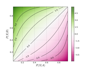
One approach to inference uses large sample approximations to the sampling distribution of the log odds ratio (the natural logarithm of the odds ratio). If we use the joint probability notation defined above, the population log odds ratio is

{\log \left({\frac {p_{11}p_{00}}{p_{01}p_{10}}}\right)=\log(p_{11})+\log(p_{00}{\big )}-\log(p_{10})-\log(p_{01})}.\,

If we observe data in the form of a contingency table

{\begin{array}{c|cc}&Y=1&Y=0\\\hline X=1&n_{11}&n_{10}\\X=0&n_{01}&n_{00}\end{array}}

then the probabilities in the joint distribution can be estimated as

{\begin{array}{c|cc}&Y=1&Y=0\\\hline X=1&{\hat {p}}_{11}&{\hat {p}}_{10}\\X=0&{\hat {p}}_{01}&{\hat {p}}_{00}\end{array}}

where $︿ p ij = n ij / n$ , with $n = n 11 + n 10 + n 01 + n 00$ being the sum of all four cell counts. The sample log odds ratio is

{L=\log \left({\dfrac {{\hat {p}}_{11}{\hat {p}}_{00}}{{\hat {p}}_{10}{\hat {p}}_{01}}}\right)=\log \left({\dfrac {n_{11}n_{00}}{n_{10}n_{01}}}\right)}

.

The distribution of the log odds ratio is approximately normal with:

L\ \sim \ {\mathcal {N}}(\log(OR),\,\sigma ^{2}).\,

The standard error for the log odds ratio is approximately

{{\rm {SE}}={\sqrt {{\dfrac {1}{n_{11}}}+{\dfrac {1}{n_{10}}}+{\dfrac {1}{n_{01}}}+{\dfrac {1}{n_{00}}}}}}

.

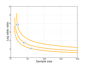
This is an asymptotic approximation, and will not give a meaningful result if any of the cell counts are very small. If L is the sample log odds ratio, an approximate 95% confidence interval for the population log odds ratio is $L \pm 1.96SE$ .[3] This can be mapped to $exp(L - 1.96SE), exp(L + 1.96SE)$ to obtain a 95% confidence interval for the odds ratio. If we wish to test the hypothesis that the population odds ratio equals one, the two-sided p-value is $2 P (Z < - | L | /SE)$ , where P denotes a probability, and Z denotes a standard normal random variable.

An alternative approach to inference for odds ratios looks at the distribution of the data conditionally on the marginal frequencies of X and Y. An advantage of this approach is that the sampling distribution of the odds ratio can be expressed exactly.

Role in logistic regression

Logistic regression is one way to generalize the odds ratio beyond two binary variables. Suppose we have a binary response variable Y and a binary predictor variable X, and in addition we have other predictor variables Z₁, ..., Z_p that may or may not be binary. If we use multiple logistic regression to regress Y on X, Z₁, ..., Z_p, then the estimated coefficient ${\hat {\beta }}_{x}$ for X is related to a conditional odds ratio. Specifically, at the population level

\exp(\beta _{x})={\frac {P(Y=1\mid X=1,Z_{1},\ldots ,Z_{p})/P(Y=0\mid X=1,Z_{1},\ldots ,Z_{p})}{P(Y=1\mid X=0,Z_{1},\ldots ,Z_{p})/P(Y=0\mid X=0,Z_{1},\ldots ,Z_{p})}},

so $\exp({\hat {\beta }}_{x})$ is an estimate of this conditional odds ratio. The interpretation of $\exp({\hat {\beta }}_{x})$ is as an estimate of the odds ratio between Y and X when the values of Z₁, ..., Z_p are held fixed.

Insensitivity to the type of sampling

If the data form a "population sample", then the cell probabilities $\land p ij$ are interpreted as the frequencies of each of the four groups in the population as defined by their X and Y values. In many settings it is impractical to obtain a population sample, so a selected sample is used. For example, we may choose to sample units with $X = 1$ with a given probability f, regardless of their frequency in the population (which would necessitate sampling units with $X = 0$ with probability $1 - f$ ). In this situation, our data would follow the following joint probabilities:

{\begin{array}{c|cc}&Y=1&Y=0\\\hline X=1&{\frac {fp_{11}}{p_{11}+p_{10}}}&{\frac {fp_{10}}{p_{11}+p_{10}}}\\X=0&{\frac {(1-f)p_{01}}{p_{01}+p_{00}}}&{\frac {(1-f)p_{00}}{p_{01}+p_{00}}}\end{array}}

The odds ratio $p 11 p 00 / p 01 p 10$ for this distribution does not depend on the value of f. This shows that the odds ratio (and consequently the log odds ratio) is invariant to non-random sampling based on one of the variables being studied. Note however that the standard error of the log odds ratio does depend on the value of f.

This fact is exploited in two important situations:

Suppose it is inconvenient or impractical to obtain a population sample, but it is practical to obtain a convenience sample of units with different X values, such that within the $X = 0$ and $X = 1$ subsamples the Y values are representative of the population (i.e. they follow the correct conditional probabilities).
Suppose the marginal distribution of one variable, say X, is very skewed. For example, if we are studying the relationship between high alcohol consumption and pancreatic cancer in the general population, the incidence of pancreatic cancer would be very low, so it would require a very large population sample to get a modest number of pancreatic cancer cases. However we could use data from hospitals to contact most or all of their pancreatic cancer patients, and then randomly sample an equal number of subjects without pancreatic cancer (this is called a "case-control study").

In both these settings, the odds ratio can be calculated from the selected sample, without biasing the results relative to what would have been obtained for a population sample.

Use in quantitative research

Due to the widespread use of logistic regression, the odds ratio is widely used in many fields of medical and social science research. The odds ratio is commonly used in survey research, in epidemiology, and to express the results of some clinical trials, such as in case-control studies. It is often abbreviated "OR" in reports. When data from multiple surveys is combined, it will often be expressed as "pooled OR".

Relation to relative risk

In clinical studies, as well as in some other settings, the parameter of greatest interest is often the relative risk rather than the odds ratio. The relative risk is best estimated using a population sample, but if the rare disease assumption holds, the odds ratio is a good approximation to the relative risk — the odds is p / (1 − p), so when p moves towards zero, 1 − p moves towards 1, meaning that the odds approaches the risk, and the odds ratio approaches the relative risk.[4] When the rare disease assumption does not hold, the odds ratio can overestimate the relative risk.[5][6][7]

If the absolute risk in the control group is available, conversion between the two is calculated by:[5]

RR\approx {\frac {OR}{1-R_{C}+(R_{C}\times OR)}}

where:

RR = relative risk
OR = odds ratio
R_C = absolute risk in the unexposed group, given as a fraction (for example: fill in 10% risk as 0.1)

Confusion and exaggeration

Odds ratios have often been confused with relative risk in medical literature. For non-statisticians, the odds ratio is a difficult concept to comprehend, and it gives a more impressive figure for the effect.[8] However, most authors consider that the relative risk is readily understood.[9] In one study, members of a national disease foundation were actually 3.5 times more likely than nonmembers to have heard of a common treatment for that disease – but the odds ratio was 24 and the paper stated that members were ‘more than 20-fold more likely to have heard of’ the treatment.[10] A study of papers published in two journals reported that 26% of the articles that used an odds ratio interpreted it as a risk ratio.[11]

This may reflect the simple process of uncomprehending authors choosing the most impressive-looking and publishable figure.[9] But its use may in some cases be deliberately deceptive.[12] It has been suggested that the odds ratio should only be presented as a measure of effect size when the risk ratio cannot be estimated directly.[8]

Invertibility and invariance

The odds ratio has another unique property of being directly mathematically invertible whether analyzing the OR as either disease survival or disease onset incidence – where the OR for survival is direct reciprocal of 1/OR for risk. This is known as the 'invariance of the odds ratio'. In contrast, the relative risk does not possess this mathematical invertible property when studying disease survival vs. onset incidence. This phenomenon of OR invertibility vs. RR non-invertibility is best illustrated with an example:

Suppose in a clinical trial, one has an adverse event risk of 4/100 in drug group, and 2/100 in placebo... yielding a RR=2 and OR=2.04166 for drug-vs-placebo adverse risk. However, if analysis was inverted and adverse events were instead analyzed as event-free survival, then the drug group would have a rate of 96/100, and placebo group would have a rate of 98/100—yielding a drug-vs-placebo a RR=0.9796 for survival, but an OR=0.48979. As one can see, a RR of 0.9796 is clearly not the reciprocal of a RR of 2. In contrast, an OR of 0.48979 is indeed the direct reciprocal of an OR of 2.04166.

This is again what is called the 'invariance of the odds ratio', and why a RR for survival is not the same as a RR for risk, while the OR has this symmetrical property when analyzing either survival or adverse risk. The danger to clinical interpretation for the OR comes when the adverse event rate is not rare, thereby exaggerating differences when the OR rare-disease assumption is not met. On the other hand, when the disease is rare, using a RR for survival (e.g. the RR=0.9796 from above example) can clinically hide and conceal an important doubling of adverse risk associated with a drug or exposure.

Estimators of the odds ratio

Sample odds ratio

The sample odds ratio n₁₁n₀₀ / n₁₀n₀₁ is easy to calculate, and for moderate and large samples performs well as an estimator of the population odds ratio. When one or more of the cells in the contingency table can have a small value, the sample odds ratio can be biased and exhibit high variance.

Alternative estimators

A number of alternative estimators of the odds ratio have been proposed to address limitations of the sample odds ratio. One alternative estimator is the conditional maximum likelihood estimator, which conditions on the row and column margins when forming the likelihood to maximize (as in Fisher's exact test).[13] Another alternative estimator is the Mantel–Haenszel estimator.

Numerical examples

The following four contingency tables contain observed cell counts, along with the corresponding sample odds ratio (OR) and sample log odds ratio (LOR):

	OR = 1, LOR = 0		OR = 1, LOR = 0		OR = 4, LOR = 1.39		OR = 0.25, LOR = −1.39
	Y = 1	Y = 0	Y = 1	Y = 0	Y = 1	Y = 0	Y = 1	Y = 0
X = 1	10	10	100	100	20	10	10	20
X = 0	5	5	50	50	10	20	20	10

The following joint probability distributions contain the population cell probabilities, along with the corresponding population odds ratio (OR) and population log odds ratio (LOR):

	OR = 1, LOR = 0		OR = 1, LOR = 0		OR = 16, LOR = 2.77		OR = 0.67, LOR = −0.41
	Y = 1	Y = 0	Y = 1	Y = 0	Y = 1	Y = 0	Y = 1	Y = 0
X = 1	0.2	0.2	0.4	0.4	0.4	0.1	0.1	0.3
X = 0	0.3	0.3	0.1	0.1	0.1	0.4	0.2	0.4

Numerical example

	Example of risk reduction
	Experimental group (E)	Control group (C)	Total
Events (E)	EE = 15	CE = 100	115
Non-events (N)	EN = 135	CN = 150	285
Total subjects (S)	ES = EE + EN = 150	CS = CE + CN = 250	400
Event rate (ER)	EER = EE / ES = 0.1, or 10%	CER = CE / CS = 0.4, or 40%

Equation	Variable	Abbr.	Value
CER - EER	absolute risk reduction	ARR	0.3, or 30%
(CER - EER) / CER	relative risk reduction	RRR	0.75, or 75%
1 / (CER − EER)	number needed to treat	NNT	3.33
EER / CER	risk ratio	RR	0.25
(EE / EN) / (CE / CN)	odds ratio	OR	0.167
(CER - EER) / CER	preventable fraction among the unexposed	PFu	0.75

Related statistics

There are various other summary statistics for contingency tables that measure association between two events, such as Yule's Y, Yule's Q; these two are normalized so they are 0 for independent events, 1 for perfectly correlated, −1 for perfectly negatively correlated. Edwards (1963) studied these and argued that measures of association must be a function of the odds ratio, which he referred to as the cross-ratio.

References

Citations

Szumilas, Magdalena (August 2010). "Explaining Odds Ratios". Journal of the Canadian Academy of Child and Adolescent Psychiatry. 19 (3): 227–229. ISSN 1719-8429. PMC 2938757. PMID 20842279.
LaMorte WW (May 13, 2013), Case-Control Studies, Boston University School of Public Health, retrieved 2013-09-02
Morris JA, Gardner MJ (May 1988). "Calculating confidence intervals for relative risks (odds ratios) and standardised ratios and rates". British Medical Journal (Clinical Research Ed.). 296 (6632): 1313–6. doi:10.1136/bmj.296.6632.1313. PMC 2545775. PMID 3133061.
Viera AJ (July 2008). "Odds ratios and risk ratios: what's the difference and why does it matter?". Southern Medical Journal. 101 (7): 730–4. doi:10.1097/SMJ.0b013e31817a7ee4. PMID 18580722.
Zhang J, Yu KF (November 1998). "What's the relative risk? A method of correcting the odds ratio in cohort studies of common outcomes". JAMA. 280 (19): 1690–1. doi:10.1001/jama.280.19.1690. PMID 9832001.
Robbins AS, Chao SY, Fonseca VP (October 2002). "What's the relative risk? A method to directly estimate risk ratios in cohort studies of common outcomes". Annals of Epidemiology. 12 (7): 452–4. doi:10.1016/S1047-2797(01)00278-2. PMID 12377421.
Nurminen M (August 1995). "To use or not to use the odds ratio in epidemiologic analyses?". European Journal of Epidemiology. 11 (4): 365–71. doi:10.1007/BF01721219. PMID 8549701.
Taeger D, Sun Y, Straif K (10 August 1998). "On the use, misuse and interpretation of odds ratios".
A'Court C, Stevens R, Heneghan C (March 2012). "Against all odds? Improving the understanding of risk reporting". The British Journal of General Practice. 62 (596): e220–3. doi:10.3399/bjgp12X630223. PMC 3289830. PMID 22429441.
Nijsten T, Rolstad T, Feldman SR, Stern RS (January 2005). "Members of the national psoriasis foundation: more extensive disease and better informed about treatment options". Archives of Dermatology. 141 (1): 19–26. doi:10.1001/archderm.141.1.19. PMID 15655138.
Holcomb, W (2001). "An odd measure of risk: Use and misuse of the odds ratio". Obstetrics & Gynecology. 98 (4): 685–688. doi:10.1016/S0029-7844(01)01488-0.
Taylor HG (January 1975). "Social perception of the mentally retarded". Journal of Clinical Psychology. 31 (1): 100–2. doi:10.1136/bmj.316.7136.989. PMC 1112884. PMID 9550961.
Rothman KJ, Greenland S, Lash TL (2008). Modern Epidemiology. Lippincott Williams & Wilkins. ISBN 978-0-7817-5564-1.

Sources

Edwards, A. W. F. (1963). "The Measure of Association in a 2 × 2 Table". Journal of the Royal Statistical Society. A (General). 126 (1): 109–114. doi:10.2307/2982448. JSTOR 2982448.

External links

This article is issued from Wikipedia. The text is licensed under Creative Commons - Attribution - Sharealike. Additional terms may apply for the media files.

[1] Szumilas, Magdalena (August 2010). "Explaining Odds Ratios". Journal of the Canadian Academy of Child and Adolescent Psychiatry. 19 (3): 227–229. ISSN 1719-8429. PMC 2938757. PMID 20842279.

[BUCaseControl-2] LaMorte WW (May 13, 2013), Case-Control Studies, Boston University School of Public Health, retrieved 2013-09-02

[pmid3133061-3] Morris JA, Gardner MJ (May 1988). "Calculating confidence intervals for relative risks (odds ratios) and standardised ratios and rates". British Medical Journal (Clinical Research Ed.). 296 (6632): 1313–6. doi:10.1136/bmj.296.6632.1313. PMC 2545775. PMID 3133061.

[pmid18580722-4] Viera AJ (July 2008). "Odds ratios and risk ratios: what's the difference and why does it matter?". Southern Medical Journal. 101 (7): 730–4. doi:10.1097/SMJ.0b013e31817a7ee4. PMID 18580722.

[pmid9832001-5] Zhang J, Yu KF (November 1998). "What's the relative risk? A method of correcting the odds ratio in cohort studies of common outcomes". JAMA. 280 (19): 1690–1. doi:10.1001/jama.280.19.1690. PMID 9832001.

[pmid12377421-6] Robbins AS, Chao SY, Fonseca VP (October 2002). "What's the relative risk? A method to directly estimate risk ratios in cohort studies of common outcomes". Annals of Epidemiology. 12 (7): 452–4. doi:10.1016/S1047-2797(01)00278-2. PMID 12377421.

[7] Nurminen M (August 1995). "To use or not to use the odds ratio in epidemiologic analyses?". European Journal of Epidemiology. 11 (4): 365–71. doi:10.1007/BF01721219. PMID 8549701.

[bmj.com-8] Taeger D, Sun Y, Straif K (10 August 1998). "On the use, misuse and interpretation of odds ratios".

[ACourt-9] A'Court C, Stevens R, Heneghan C (March 2012). "Against all odds? Improving the understanding of risk reporting". The British Journal of General Practice. 62 (596): e220–3. doi:10.3399/bjgp12X630223. PMC 3289830. PMID 22429441.

[10] Nijsten T, Rolstad T, Feldman SR, Stern RS (January 2005). "Members of the national psoriasis foundation: more extensive disease and better informed about treatment options". Archives of Dermatology. 141 (1): 19–26. doi:10.1001/archderm.141.1.19. PMID 15655138.

[11] Holcomb, W (2001). "An odd measure of risk: Use and misuse of the odds ratio". Obstetrics & Gynecology. 98 (4): 685–688. doi:10.1016/S0029-7844(01)01488-0.

[12] Taylor HG (January 1975). "Social perception of the mentally retarded". Journal of Clinical Psychology. 31 (1): 100–2. doi:10.1136/bmj.316.7136.989. PMC 1112884. PMID 9550961.

[13] Rothman KJ, Greenland S, Lash TL (2008). Modern Epidemiology. Lippincott Williams & Wilkins. ISBN 978-0-7817-5564-1.