Compartmental models in epidemiology
Compartmental models are a technique used to simplify the mathematical modelling of infectious disease. The population is divided into compartments, with the assumption that every individual in the same compartment has the same characteristics. Its origin is in the early 20th century, with an important early work being that of Kermack and McKendrick in 1927.[1]
The models are usually investigated through ordinary differential equations (which are deterministic), but can also be viewed in a stochastic framework, which is more realistic but also more complicated to analyse.
Compartmental models may be used to predict properties of how a disease spreads, for example the prevalence (total number of infected) or the duration of an epidemic. Also, the model allows for understanding how different situations may affect the outcome of the epidemic, e.g., what the most efficient technique is for issuing a limited number of vaccines in a given population.
The SIR model
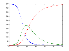
The SIR model is one of the simplest compartmental models, and many models are derivations of this basic form. The model consists of three compartments– S for the number susceptible, I for the number of infectious, and R for the number recovered (or immune). This model is reasonably predictive for infectious diseases which are transmitted from human to human, and where recovery confers lasting resistance, such as measles, mumps and rubella.
These variables (S, I, and R) represent the number of people in each compartment at a particular time. To represent that the number of susceptible, infected and recovered individuals may vary over time (even if the total population size remains constant), we make the precise numbers a function of t (time): S(t), I(t) and R(t). For a specific disease in a specific population, these functions may be worked out in order to predict possible outbreaks and bring them under control.
The SIR model is dynamic in three senses
As implied by the variable function of t, the model is dynamic in that the numbers in each compartment may fluctuate over time. The importance of this dynamic aspect is most obvious in an endemic disease with a short infectious period, such as measles in the UK prior to the introduction of a vaccine in 1968. Such diseases tend to occur in cycles of outbreaks due to the variation in number of susceptibles (S(t)) over time. During an epidemic, the number of susceptible individuals falls rapidly as more of them are infected and thus enter the infectious and recovered compartments. The disease cannot break out again until the number of susceptibles has built back up as a result of offspring being born into the susceptible compartment.
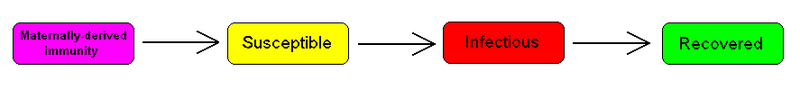
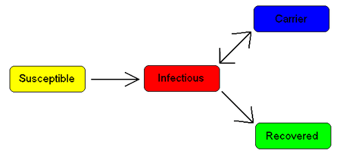
Each member of the population typically progresses from susceptible to infectious to recovered. This can be shown as a flow diagram in which the boxes represent the different compartments and the arrows the transition between compartments, i.e.

Transition rates
For the full specification of the model, the arrows should be labeled with the transition rates between compartments. Between S and I, the transition rate is βI, where β is the average number of contacts per person times the probability of disease transmission in a contact between a susceptible and an infectious subject.
Between I and R, the transition rate is γ (simply the rate of recovery or death). If the duration of the infection is denoted D, then γ = 1/D, since an individual experiences one recovery in D units of time.
It's assumed that the permanence of each single subject in the epidemic states is a random variable with exponential distribution. More complex and realistic distributions (such as Erlang distribution) can be equally used with few modifications.
Bio-mathematical deterministic treatment of the SIR model
The SIR model without vital dynamics
The dynamics of an epidemic, for example the flu, are often much faster than the dynamics of birth and death, therefore, birth and death are often omitted in simple compartmental models. The SIR system without so-called vital dynamics (birth and death, sometimes called demography) described above can be expressed by the following set of ordinary differential equations:[2]
- ,

- ,

- .

Where is the stock of susceptible population, is the stock of infected, and is the stock of recovered population.


This model was for the first time proposed by O. Kermack and Anderson Gray McKendrick as a special case of what we now call Kermack-McKendrick theory, and followed work McKendrick had done with Ronald Ross.
This system is non-linear, and does not admit a generic analytic solution. Nevertheless, significant results can be derived analytically, and with Monte Carlo methods, such as the Gillespie algorithm.
Firstly note that from:
- ,

it follows that:
- ,

expressing in mathematical terms the constancy of population . Note that the above relationship implies that one need only study the equation for two of the three variables.

Secondly, we note that the dynamics of the infectious class depends on the following ratio:
- ,

the so-called basic reproduction number (also called basic reproduction ratio). This ratio is derived as the expected number of new infections (these new infections are sometimes called secondary infections) from a single infection in a population where all subjects are susceptible.[3][4] This idea can probably be more readily seen if we say that the typical time between contacts is , and the typical time until recovery is . From here it follows that, on average, the number of contacts by an infected individual with others before the infected has recovered is:


By dividing the first differential equation by the third, separating the variables and integrating we get
- ,

(where and are the initial numbers of, respectively, susceptible and removed subjects). Thus, in the limit , the proportion of recovered individuals obeys the following transcendental equation


- .

This equation shows that at the end of an epidemic, unless , not all individuals of the population have recovered, so some must remain susceptible. This means that the end of an epidemic is caused by the decline in the number of infected individuals rather than an absolute lack of susceptible subjects. The role of the basic reproduction number is extremely important. In fact, upon rewriting the equation for infectious individuals as follows:

- ,

it yields that if:

then:

i.e., there will be a proper epidemic outbreak with an increase of the number of the infectious (which can reach a considerable fraction of the population). On the contrary, if

then

i.e., independently from the initial size of the susceptible population the disease can never cause a proper epidemic outbreak. As a consequence, it is clear that the basic reproduction number is extremely important.
The force of infection
Note that in the above model the function:

models the transition rate from the compartment of susceptible individuals to the compartment of infectious individuals, so that it is called the force of infection. However, for large classes of communicable diseases it is more realistic to consider a force of infection that does not depend on the absolute number of infectious subjects, but on their fraction (with respect to the total constant population ):

Capasso and, afterwards, other authors have proposed nonlinear forces of infection to model more realistically the contagion process.
Exact analytical solutions to the SIR model
In 2014, Harko T. et al.[5] derived an exact analytical solution to the SIR model. In the without vital dynamics setup, for , etc., it corresponds to the following time parametrization


for , , with initial conditions , where satisfies . By the transcendental equation for above, it follows that , if and .


An equivalent analytical solution was found by Miller[6][7] yields


Here can be interpreted as the expected number of transmissions an individual has received by time . The two solutions are related by .


Effectively the same result can be found in the original work by Kermack and McKendrick.[8]
The SIR model with vital dynamics and constant population
Considering a population characterized by a death rate and birth rate , and where a communicable disease is spreading. The model with mass-action transmission is:


for which the disease-free equilibrium (DFE) is:

In this case, we can derive a basic reproduction number :

which has threshold properties. In fact, independently from biologically meaningful initial values, one can show that:


The point EE is called the Endemic Equilibrium. With heuristic arguments, one may show that may be read as the average number of infections caused by a single infectious subject in a wholly susceptible population, the above relationship biologically means that if this number is less or equal than one the disease goes extinct, whereas if this number is greater than one the disease will remain permanently endemic in the population.

The SIS model
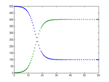
Some infections, for example those from the common cold and influenza, do not confer any long lasting immunity. Such infections do not give immunization upon recovery from infection, and individuals become susceptible again.

We have the model:


Note that denoting with N the total population it holds that: it follows that:


i.e. the dynamics of infectious is ruled by a logistic equation, so that :


It is possible to find an analytical solution to this model (by making a transformation of variables: and substituting this into the mean-field equations),[9] such that the basic reproduction rate is greater than unity. The solution is given as


where is the endemic infected population, , and . As the system is assumed to be closed, the susceptible population is then .


Elaborations on the basic SIR model
The MSIR model
For many infections, including measles, babies are not born into the susceptible compartment but are immune to the disease for the first few months of life due to protection from maternal antibodies (passed across the placenta and additionally through colostrum). This is called passive immunity. This added detail can be shown by including an M class (for maternally derived immunity) at the beginning of the model
To indicate this mathematically, an additional compartment is added, M(t), which results in the following differential equations:


Carrier state
Some people who have had an infectious disease such as tuberculosis never completely recover and continue to carry the infection, whilst not suffering the disease themselves. They may then move back into the infectious compartment and suffer symptoms (as in tuberculosis) or they may continue to infect others in their carrier state, while not suffering symptoms. The most famous example of this is probably Mary Mallon, who infected 22 people with typhoid fever. The carrier compartment is labelled C.
The SEIR model
For many important infections there is a significant incubation period during which the individual has been infected but is not yet infectious themselves. During this period the individual is in compartment E (for exposed).

Assuming that the incubation period is a random variable with exponential distribution with parameter a (i.e. the average incubation period is ), and also assuming the presence of vital dynamics with birth rate equal to death rate, we have the model:


We have , but this is only constant because of the (degenerate) assumption that birth and death rates are equal; in general is a variable.

For this model, the basic reproduction number is:

Similarly to the SIR model, also in this case we have a Disease-Free-Equilibrium (N,0,0,0) and an Endemic Equilibrium EE, and one can show that, independently form biologically meaningful initial conditions

it holds that:


In case of periodically varying contact rate the condition for the global attractiveness of DFE is that the following linear system with periodic coefficients:


is stable (i.e. it has its Floquet's eigenvalues inside the unit circle in the complex plane).
The SEIS model
The SEIS model takes into consideration the exposed or latent period of the disease, giving an additional compartment, E(t).

In this model an infection does not leave any immunity thus individuals that have recovered return to being susceptible again, moving back into the S(t) compartment. The following differential equations describe this model:


The MSEIR model
For the case of a disease, with the factors of passive immunity, and a latency period there is the MSEIR model.


The MSEIRS model
An MSEIRS model is similar to the MSEIR, but the immunity in the R class would be temporary, so that individuals would regain their susceptibility when the temporary immunity ended.

Variable contact rates and pluriannual or chaotic epidemics
It is well known that the probability of getting a disease is not constant in the time. Some diseases are seasonal, such as the common cold viruses, which are more prevalent during winter. With childhood diseases, such as measles, mumps, and rubella, there is a strong correlation with the school calendar, so that during the school holidays the probability of getting such a disease dramatically decreases.
As a consequence, for many classes of diseases one should consider a force of infection with periodically ('seasonal') varying contact rate

with period T equal to one year.
Thus, our model becomes


(the dynamics of recovered easily follows from ), i.e. a nonlinear set of differential equations with periodically varying parameters. It is well known that this class of dynamical systems may undergo very interesting and complex phenomena of nonlinear parametric resonance. It is easy to see that if:


whereas if the integral is greater than one the disease will not die out and there may be such resonances. For example, considering the periodically varying contact rate as the 'input' of the system one has that the output is a periodic function whose period is a multiple of the period of the input. This allowed to give a contribution to explain the poly-annual (typically biennial) epidemic outbreaks of some infectious diseases as interplay between the period of the contact rate oscillations and the pseudo-period of the damped oscillations near the endemic equilibrium. Remarkably, in some cases the behavior may also be quasi-periodic or even chaotic.
Modelling vaccination
The SIR model can be modified to model vaccination. Typically these introduce an additional compartment to the SIR model, , for vaccinated individuals. Below are some examples.

Vaccinating newborns
In presence of a communicable diseases, one of main tasks is that of eradicating it via prevention measures and, if possible, via the establishment of a mass vaccination program. Consider a disease for which the newborn are vaccinated (with a vaccine giving lifelong immunity) at a rate :


where is the class of vaccinated subjects. It is immediate to show that:

thus we shall deal with the long term behavior of and , for which it holds that:


In other words, if

the vaccination program is not successful in eradicating the disease, on the contrary it will remain endemic, although at lower levels than the case of absence of vaccinations. This means that the mathematical model suggests that for a disease whose basic reproduction number may be as high as 18 one should have to vaccinate 94.4% of newborns in order to eradicate the disease.
Vaccination and information
Modern societies are facing the challenge of "rational" exemption, i.e. the family's decision to not vaccinate children as a consequence of a "rational" comparison between the perceived risk from infection and that from getting damages from the vaccine. In order to assess whether this behavior is really rational, i.e. if it can equally lead to the eradication of the disease, one may simply assume that the vaccination rate is an increasing function of the number of infectious subjects:

In such a case the eradication condition becomes:

i.e. the baseline vaccination rate should be greater than the "mandatory vaccination" threshold, which, in case of exemption, cannot hold. Thus, "rational" exemption might be myopic since it is based only on the current low incidence due to high vaccine coverage, instead taking into account future resurgence of infection due to coverage decline.
Vaccination of non newborns
In case there also are vaccinations of non newborn at a rate ρ the equation for the susceptible and vaccinated subject has to be modified as follows:


leading to the following eradication condition:

Pulse vaccination strategy
This strategy repeatedly vaccinates a defined age-cohort (such as young children or the elderly) in a susceptible population over time. Using this strategy, the block of susceptible individuals is then immediately removed, making it possible to eliminate an infectious disease, (such as measles), from the entire population. Every T time units a constant fraction p of susceptible subjects is vaccinated in a relatively short (with respect to the dynamics of the disease) time. This leads to the following impulsive differential equations for the susceptible and vaccinated subjects:


It is easy to see that by setting I = 0 one obtains that the dynamics of the susceptible subjects is given by:

and that the eradication condition is:

The influence of age: age-structured models
Age has a deep influence on the disease spread rate in a population, especially the contact rate. This rate summarizes the effectiveness of contacts between susceptible and infectious subjects. Taking into account the ages of the epidemic classes (to limit ourselves to the susceptible-infectious-removed scheme) such that:


(where is the maximum admissible age)and their dynamics is not described, as one might think, by "simple" partial differential equations, but by integro-differential equations:


where:

is the force of infection, which, of course, will depend, though the contact kernel on the interactions between the ages.

Complexity is added by the initial conditions for newborns (i.e. for a=0), that are straightforward for infectious and removed:

but that are nonlocal for the density of susceptible newborns:

where are the fertilities of the adults.

Moreover, defining now the density of the total population one obtains:


In the simplest case of equal fertilities in the three epidemic classes, we have that in oder to have demographic equilibrium the following necessary and sufficient condition linking the fertility with the mortality must hold:


and the demographic equilibrium is

automatically ensuring the existence of the disease-free solution:

A basic reproduction number can be calculated as the spectral radius of an appropriate functional operator.
Other considerations within compartmental epidemic models
Vertical transmission
In the case of some diseases such as AIDS and Hepatitis B, it is possible for the offspring of infected parents to be born infected. This transmission of the disease down from the mother is called Vertical Transmission. The influx of additional members into the infected category can be considered within the model by including a fraction of the newborn members in the infected compartment.[10]
Vector transmission
Diseases transmitted from human to human indirectly, i.e. malaria spread by way of mosquitoes, are transmitted through a vector. In these cases, the infection transfers from human to insect and an epidemic model must include both species, generally requiring many more compartments than a model for direct transmission.[10] For more information on this type of model see the reference Population Dynamics of Infectious Diseases: Theory and Applications, by R. M. Anderson.[11]
Others
Other occurrences which may need to be considered when modeling an epidemic include things such as the following:[10]
- • Nonhomogeneous mixing
- • Variable infectivity
- • Distributions that are spatially non-uniform
- • Diseases caused by macroparasites
Deterministic versus stochastic epidemic models
It is important to stress that the deterministic models presented here are valid only in case of sufficiently large populations, and as such should be used cautiously.[12]
To be more precise, these models are only valid in the thermodynamic limit, where the population is effectively infinite. In stochastic models, the long-time endemic equilibrium derived above, does not hold, as there is a finite probability that the number of infected individuals drops below one in a system. In a true system then, the pathogen may not propagate, as no host will be infected. But, in deterministic mean-field models, the number of infecteds can take on real, namely, non-integer values of infected hosts, and the pathogen may still persist in the system with a finite number of infected hosts, less than one but greater than zero.
See also
- Mathematical modelling in epidemiology
- Modifiable Areal Unit Problem
- Next-generation matrix
- Risk assessment
- Attack rate
References
- Kermack WO, McKendrick AG (August 1, 1927). "A Contribution to the Mathematical Theory of Epidemics". Proceedings of the Royal Society A. 115 (772): 700–721. doi:10.1098/rspa.1927.0118.
- Hethcote H (2000). "The Mathematics of Infectious Diseases" (PDF). SIAM Review. 42 (4): 599–653. doi:10.1137/s0036144500371907.
- Bailey, Norman T. J. (1975). The mathematical theory of infectious diseases and its applications (2nd ed.). London: Griffin. ISBN 0-85264-231-8.
- Sonia Altizer; Nunn, Charles (2006). Infectious diseases in primates: behavior, ecology and evolution. Oxford Series in Ecology and Evolution. Oxford [Oxfordshire]: Oxford University Press. ISBN 0-19-856585-2.
- Harko T., Lobo F.S.N., and Mak M.K. (2014). "Exact analytical solutions of the Susceptible-Infected-Recovered (SIR) epidemic model and of the SIR model with equal death and birth rates". Applied Mathematics and Computation. 236: 184–194. doi:10.1016/j.amc.2014.03.030.CS1 maint: multiple names: authors list (link)
- Miller, J.C. (2012). "A note on the derivation of epidemic final sizes". Bulletin of Mathematical Biology. 74. section 4.1.
- Miller, J.C. (2017). "Mathematical models of SIR disease spread with combined non-sexual and sexual transmission routes". Infectious Disease Modelling. 2. section 2.1.3.
- Kermack WO, McKendrick AG (August 1, 1927). "A Contribution to the Mathematical Theory of Epidemics". Proceedings of the Royal Society A. 115 (772). pg 713. doi:10.1098/rspa.1927.0118.
- Hethcote, H. W. (1989). in Three Basic Epidemiological Models, Applied Mathematical Ecology, Vol. 18. Berlin: Springer.
- Brauer, F. & Castillo-Chávez, C. (2001). Mathematical Models in Population Biology and Epidemiology. NY: Springer.
- Anderson, R. M. ed. (1982) Population Dynamics of Infectious Diseases: Theory and Applications, Chapman and Hall, London-New York.
- Bartlett MS (1957). "Measles periodicity and community size". Journal of the Royal Statistical Society, Series A. 120 (1): 48–70. doi:10.2307/2342553. JSTOR 2342553.
Further reading
- May, Robert M.; Anderson, Roy M. (1991). Infectious diseases of humans: dynamics and control. Oxford [Oxfordshire]: Oxford University Press. ISBN 0-19-854040-X.
- V. Capasso, The Mathematical Structure of Epidemic Systems, Springer Verlag (1993)
- Vynnycky, E.; White, R.G. (2010). Vynnycky, E.; White, R.G. (eds.). An Introduction to Infectious Disease Modelling. Oxford: Oxford University Press. p. 368. ISBN 0-19-856576-3.