Acoustic tweezers

When a particle is suspended in the field of a sound wave, an acoustic radiation force that has risen from the scattering of the acoustic waves is exerted on the particle. This was first modeled and analyzed for incompressible particles in an ideal fluid by Louis King in 1934.[6] Yosioka and Kawasima calculated the acoustic radiation force on compressible particles in a plane wave field in 1955.[7] Gorkov summarized the previous work and proposed equations to determine the average force acting on a particle in an arbitrary acoustical field when its size is much smaller than the wavelength of the sound.[1] Recently, Bruus revisited the problem and gave detailed derivation for the acoustic radiation force.[8]

Fig. 1: acoustic radiation force on a small particle

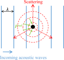
As shown in Figure 1, the acoustic radiation force on a small particle results from a non-uniform flux of momentum in the near-field region around the particle, ${\displaystyle \mathbf {\mathit {F^{rad}}} =-\nabla {\mathit {U}}}$, which is caused by the incoming acoustic waves and the scattering on the surface of the particle when acoustic waves propagate through it. For a compressible spherical particle with a diameter much smaller than the wavelength of acoustic waves in an ideal fluid, the acoustic radiation force can be calculated by ${\displaystyle \mathbf {\mathit {F^{rad}}} =-\nabla {\mathit {U}}}$, where ${\displaystyle {\mathit {U}}}$ is a given quantity, also called acoustic potential energy.[1][8] The acoustic potential energy is expressed as:

${\displaystyle U={V_{0}}({{\overline {p_{in}^{2}}} \over {2{\rho _{f}}c_{f}^{2}}}{f_{1}}-{{3{\rho _{f}}{\overline {v_{in}^{2}}}} \over 4}{f_{2}})}$

where

• ${\displaystyle {\mathit {V_{\mathit {0}}}}}$ is the particle volume,
• ${\displaystyle {\mathit {p_{\mathit {in}}}}}$ is the acoustic pressure,
• ${\displaystyle {\mathit {v_{\mathit {in}}}}}$ is the velocity of acoustic particles,
• ${\displaystyle {\mathit {\rho }}_{\mathit {f}}}$ is the fluid mass density,
• ${\displaystyle {\mathit {c_{\mathit {f}}}}}$ is the speed of sound of the fluid,
• ${\displaystyle {\overline {<*>}}}$ is the time-average term, ${\displaystyle {1 \over T}\int \limits _{0}^{T}{(*)}dt}$

The coefficients ${\displaystyle {\mathit {f_{\mathit {1}}}}}$ and ${\displaystyle {\mathit {f_{\mathit {2}}}}}$ can be calculated by ${\displaystyle {f_{1}}=1-{{{\rho _{f}}c_{f}^{2}} \over {{\rho _{p}}c_{p}^{2}}}}$ and ${\displaystyle {f_{2}}={{2({\rho _{p}}-{\rho _{f}})} \over {2{\rho _{p}}+{\rho _{f}}}}}$

where

• ${\displaystyle {\mathit {\rho }}_{\mathit {p}}}$ is the mass density of the particle,
• ${\displaystyle {\mathit {c}}_{\mathit {p}}}$ is the speed of sound of the particle.

The standing waves can form a stable acoustic potential energy field, so they are able to create stable acoustic radiation force distribution, which is desirable for many acoustic tweezers applications. For one-dimension planar standing waves, the acoustic fields are given by:[8]

${\displaystyle {A_{in}}(x,t)={{-P_{0}} \over {{\rho _{f}}\omega }}\sin(kx)\sin(\omega t)}$,

${\displaystyle {p_{in}}(x,t)={P_{0}}\cos(kx)\sin(\omega t)}$,

${\displaystyle {\textbf {v}}_{\textbf {in}}(x,t)={\frac {-P_{0}}{\rho _{f}c_{f}}}\sin(kx)\cos(\omega t)){\textbf {e}}_{\textbf {x}}}$,

where

• ${\displaystyle {\mathit {A_{\mathit {in}}}}}$ is the displacement of acoustic particle,
• ${\displaystyle {\mathit {P_{\mathit {0}}}}}$ is the acoustic pressure amplitude,
• ${\displaystyle {\mathit {\omega }}}$ is the angular velocity,
• ${\displaystyle {\mathit {k}}}$ is the wave number.

With these fields, the time-average terms can be obtained. These are:

${\displaystyle {\overline {p_{in}^{2}}}={1 \over 2}P_{0}^{2}{\cos ^{2}}(kx)}$,

${\displaystyle {\overline {v_{in}^{2}}}={{P_{0}^{2}} \over {2\rho _{f}^{2}c_{f}^{2}}}{\sin ^{2}}(kx)}$,

Thus, the acoustic potential energy is:

${\displaystyle U={V_{0}}{{P_{0}^{2}} \over {4{\rho _{f}}c_{f}^{2}}}[{\cos ^{2}}(kx){f_{1}}-{3 \over 2}{\sin ^{2}}(kx){f_{2}}]}$,

Then, the acoustic radiation force is found by differentiation:

${\displaystyle {F_{x}}^{rad}=-{\partial _{x}}U={V_{0}}k{E_{ac}}\sin(2kx)\Phi }$,

${\displaystyle {E_{ac}}={{P_{0}^{2}} \over {4{\rho _{f}}c_{f}^{2}}}}$, ${\displaystyle \Phi ={f_{1}}+{3 \over 2}{f_{2}}={{5{\rho _{p}}-2{\rho _{f}}} \over {2{\rho _{p}}+{\rho _{f}}}}-{{{\rho _{f}}c_{f}^{2}} \over {{\rho _{p}}c_{p}^{2}}}}$,

Fig. 2: positions of pressure nodes (PN) and antinodes (AN) along acoustic pressure waveform

where

• ${\displaystyle {\mathit {E_{\mathit {ac}}}}}$ is the acoustic energy density, and
• ${\displaystyle \Phi }$ is acoustophoretic contrast factor.

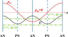
The term ${\displaystyle \sin({\mathit {2kx}})}$ shows that the radiation force period is one-half of the pressure period. Also, the contrast factor can be positive or negative depending on the properties of particles and fluid. For positive value of ${\displaystyle \Phi }$, the radiation force points from the pressure antinodes to the pressure nodes, as shown in Figure 2, and the particles will be pushed to the pressure nodes.

When multiple particles in a suspension are exposed to a standing wave field, they will not only experience acoustic radiation force, but also secondary acoustic forces caused by waves scattered by other particles. The inter-particle forces are sometimes called Bjerknes forces. A simplified equation for the inter-particle forces of identical particles is:[9][10]

${\displaystyle {F_{B}}(x)=4\pi {a^{6}}[{{{{({\rho _{p}}-{\rho _{f}})}^{2}}(3{{\cos }^{2}}\theta -1)} \over {6{\rho _{f}}{d^{4}}}}{v_{in}}^{2}(x)-{{\omega ^{2}{\rho _{f}}} \over {9{d^{2}}}}{({1 \over {{\rho _{p}}c_{p}^{2}}}-{1 \over {{\rho _{f}}c_{f}^{2}}})^{2}}p_{in}^{2}(x)]}$

where

• ${\displaystyle {\mathit {a}}}$ is the radius of the particle,
• ${\displaystyle {\mathit {d}}}$ is the distance between the particles,
• ${\displaystyle {\mathit {\theta }}}$ is the angle between the central line of the particles and the direction of propagation of the incident acoustic wave.

The sign of the force represents its direction: a negative sign for an attractive force, and a positive sign for a repulsive force. The left side of the equation depends on the acoustic particle velocity amplitude ${\displaystyle {\mathit {v}}_{\mathit {in}}({\mathit {x}})}$ and the right side depends on the acoustic pressure amplitude ${\displaystyle {\mathit {p}}_{\mathit {in}}({\mathit {x}})}$. The velocity-dependent term is repulsive when particles are aligned with wave propagation (Θ=0°), and negative when perpendicular to wave propagation (Θ=90°). The pressure-dependent term is unaffected by the particle orientation and is always attractive. In the case of a positive contrast factor, the velocity-dependent term diminishes as particles are driven to the velocity node (pressure antinode), as in the case of air bubbles and lipid vesicles. In a similar way, the pressure-dependent term diminishes as particles are driven towards the pressure node (velocity antinode), as are most solid particles in aqueous solutions.

The influence of the secondary forces is usually very weak, and only has an effect when the distance between particles is very small. It becomes important in aggregation and sedimentation applications, where particles are initially gathered in nodes by the acoustic radiation force. As interparticle distances become smaller the secondary forces assist in a further aggregation until the clusters become heavy enough for sedimentation to begin.

Acoustic streaming is a steady flow generated by a nonlinear effect in an acoustic field. Depending on the mechanisms, the acoustic streaming can be categorized into two general types, Eckert streaming and Rayleigh streaming.[11][12] Eckert streaming is driven by a time-average momentum flux created when high-amplitude acoustic waves propagate and attenuate in fluid. Rayleigh streaming, also called "boundary driven streaming", is forced by a shear viscosity close to a solid boundary. Both of the driven mechanisms come from a time-average nonlinear effect.

A perturbation approach is used to analyze the phenomenon of nonlinear acoustic streaming.[13] The governing equations for this problem are mass conservation and Navier-Stokes equations：

${\displaystyle \partial _{\mathit {t}}{\mathit {\rho }}=-\nabla \cdot ({\mathit {\rho }}{\textbf {v}})}$,

${\displaystyle {\mathit {\rho }}[\partial _{\mathit {t}}{\textbf {v}}+({\textbf {v}}\cdot \nabla ){\textbf {v}}]=-\nabla {\mathit {p}}+{\mathit {\mu }}\nabla ^{2}{\textbf {v}}+{\mathit {\beta }}{\mathit {\mu }}\nabla (\nabla \cdot {\textbf {v}}))}$

where

• ${\displaystyle {\mathit {\rho }}}$ is the density of fluid,
• ${\displaystyle {\textbf {v}}}$ is the velocity of fluid particle,
• ${\displaystyle {\mathit {p}}}$ is the pressure,
• ${\displaystyle {\mathit {\mu }}}$ is the dynamic viscosity of fluid,
• ${\displaystyle {\mathit {\beta }}}$ is the viscosity ratio.

The perturbation series can be written as ${\displaystyle p={p_{0}}+{p_{1}}+{p_{2}}}$, ${\displaystyle {\textbf {v}}={\textbf {0}}+{\textbf {v}}_{\textbf {1}}+{\textbf {v}}_{\textbf {2}}}$, ${\displaystyle {\mathit {\rho }}={\mathit {\rho }}_{0}+{\mathit {\rho }}_{1}+{\mathit {\rho }}_{2}}$, which are diminishing series with the higher-order terms much smaller than the lower-order ones.

The liquid is quiescent and homogeneous at its zero-order state. Substituting the perturbation series into the mass conservation and Navier-Stokes equation and using the relation of ${\displaystyle {p_{1}}=c_{f}^{2}{\rho _{1}}}$, the first-order equations can be obtained by collecting terms in first-order,

${\displaystyle \partial _{\mathit {t}}{\mathit {p}}_{1}=-{\mathit {\rho }}_{0}{\mathit {c}}_{\mathit {f}}^{2}\nabla \cdot {\textbf {v}}_{\textbf {1}}}$,

${\displaystyle {\mathit {\rho }}_{0}\partial _{\mathit {t}}{\textbf {v}}_{\textbf {1}}=-\nabla {\mathit {p}}_{1}+{\mathit {\mu }}\nabla ^{2}{\textbf {v}}_{\textbf {1}}+{\mathit {\beta }}{\mathit {\mu }}\nabla (\nabla \cdot {\textbf {v}}_{\textbf {1}})}$.

Similarly, the second-order equations can be found as well,

${\displaystyle \partial _{\mathit {t}}{\mathit {\rho }}_{2}=-{\mathit {\rho }}_{0}\nabla \cdot {\textbf {v}}_{\textbf {2}}-\nabla \cdot ({\mathit {\rho }}_{1}{\textbf {v}}_{\textbf {1}})}$,

${\displaystyle {\mathit {\rho }}_{0}\partial _{\mathit {t}}{\textbf {v}}_{\textbf {2}}=-\nabla {\mathit {p}}_{2}+{\mathit {\mu }}\nabla ^{2}{\textbf {v}}_{\textbf {2}}+{\mathit {\beta }}{\mathit {\mu }}\nabla (\nabla \cdot {\textbf {v}}_{\textbf {2}})-{\mathit {\rho }}_{1}\partial _{t}{\textbf {v}}_{\textbf {1}}-{\mathit {\rho }}_{0}({\textbf {v}}_{\textbf {1}}\cdot \nabla ){\textbf {v}}_{\textbf {1}}}$.

For the first-order equations, taking the time derivation of the Navier-Stokes equation and inserting the mass conservation, a combined equation can be found:

${\displaystyle {1 \over {c_{f}^{2}}}\partial _{t}^{2}{p_{1}}=[1-{{(1-\beta )\mu } \over {{\rho _{0}}c_{f}^{2}}}{\partial _{t}}]{\nabla ^{2}}{p_{1}}}$.

This is an acoustic wave equation with viscous attenuation. Physically, ${\displaystyle {\mathit {p}}_{1}}$ and ${\displaystyle {\textbf {v}}_{\textbf {1}}}$ can be interpreted as the acoustic pressure and the velocity of the acoustic particle.

The second-order equations can be considered as governing equations used to describe the motion of fluid with mass source ${\displaystyle [-\nabla \cdot ({\mathit {\rho }}_{1}{\textbf {v}}_{\textbf {1}}))]}$ and force source ${\displaystyle [-\rho _{1}\partial _{t}{\textbf {v}}_{\textbf {1}}-\rho _{0}({\textbf {v}}_{\textbf {1}}\cdot \nabla ){\textbf {v}}_{\textbf {1}}]}$. Generally, the acoustic streaming is a steady mean flow, where the response time scale is much smaller than the one of the acoustic vibration. The time-average term ${\displaystyle {\overline {{\textbf {v}}_{\textbf {2}}}}}$ is normally used to present the acoustic streaming. By using ${\displaystyle {\overline {\partial _{\mathit {t}}{\mathit {\rho }}_{2}}}=0}$, the time-average second-order equations can be obtained:

${\displaystyle {\mathit {\rho }}_{0}\nabla \cdot {\overline {{\textbf {v}}_{\textbf {2}}}}=-\nabla \cdot {\overline {({\mathit {\rho }}_{1}{\textbf {v}}_{\textbf {1}})}}}$,

${\displaystyle {\mathit {\mu }}\nabla ^{2}{\overline {{\textbf {v}}_{\textbf {2}}}}+{\mathit {\beta }}{\mathit {\mu }}\nabla (\nabla \cdot {\overline {{\textbf {v}}_{\textbf {2}}}})-{\overline {\nabla {\mathit {p}}_{2}}}={\overline {{\mathit {\rho }}_{1}\partial _{\mathit {t}}{\textbf {v}}_{\textbf {1}}}}-{\mathit {\rho }}_{0}{\overline {({\textbf {v}}_{\textbf {1}}\cdot \nabla ){\textbf {v}}_{\textbf {1}}}}}$.

Fig. 3: Cross-section of acoustic streaming around a solid cylindrical pillar

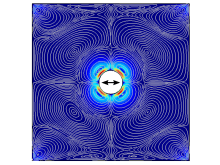
In determining the acoustic streaming, the first-order equations are most important. Since Navier-Stokes equations can only be analytically solved for simple cases, numerical methods are typically used, with the finite element method (FEM) the most common technique. It can be employed to simulate the acoustic streaming phenomena. Figure 3 is one example of acoustic streaming around a solid circular pillar, which is calculated by FEM.

As mentioned, acoustic streaming is driven by mass and force sources originating from the acoustic attenuation. However, these are not the only driven forces for acoustic streaming. The boundary vibration may also contribute, especially to "boundary driven streaming". For these cases, the boundary condition should also be processed by the perturbation approach and be imposed on the two order equations accordingly.

The motion of a suspended particle whose gravity is balanced by the buoyancy force in an acoustic field is determined by two forces: the acoustic radiation force and Stokes drag force. By applying Newton's law, the motion can be described as:

${\displaystyle {\mathit {m}}{\frac {d{\textit {u}}}{\mathit {dt}}}={\textit {F}}^{\textit {rad}}+{\textit {F}}^{\textit {drag}}}$,

${\displaystyle {\textit {F}}^{\textit {drag}}=6\pi {\mathit {a}}{\mathit {\mu }}({\textit {v}}-{\textit {u}})}$.

where

• ${\displaystyle {\textit {v}}}$ is the fluid velocity,
• ${\displaystyle {\textit {u}}}$ is the velocity of particle.

For applications in a static flow, the fluid velocity comes from the acoustic streaming. The magnitude of acoustic streaming depends on the power and frequency of the input and the properties of the fluid media. For typical acoustic-based microdevices, the operating frequency may be from the kHz to the MHz range. The vibration amplitude is in a range of 0.1 nm to 1 μm. Assuming the fluid used is water, the estimated magnitude of acoustic streaming is in the range of 1 μm/s to 1 mm/s. Thus, the acoustic streaming should be smaller than the main flow for most continuous flow applications. The drag force is mainly induced by the main flow in those applications.

Fig. 4: A proposal would use acoustic force to move red blood cells to a pressure node (center) and lipid cells to antinodes (sides).

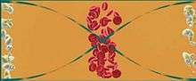
Cells with different densities and compression strengths can theoretically be separated with acoustic force. It has been suggested that acoustic tweezers could be used to separate lipid particles from red blood cells. This is a problem during cardiac surgery supported by a heart-lung machine, for which current technologies are insufficient. According to the proposal, acoustic force applied to blood plasma passing through a channel will cause red blood cells to gather in the pressure node in the center and the lipid particles to gather in antinodes at the sides (see Figure 4). At the end of the channel, the separated cells and particles exit through separate outlets.

The acoustic method might also be used to separate particles of different sizes. According to the equation of primary acoustic radiation force, larger particles experience larger forces than smaller particles. Shi et al. reported using interdigital transducers (IDTs) to generate a standing surface acoustic wave (SSAW) field with pressure nodes in the middle of a microfluidic channel, separating microparticles with different diameters.[14] When introducing a mixture of particles with different sizes from the edge of the channel, larger particles will migrate toward the middle more quickly and be collected at the center outlet. Smaller particles will not be able to migrate to the center outlet before they are collected from the side outlets. This experimental setup has also been used to separate blood components, bacteria, and hydrogel particles.[15][16][17]

Fluorescence-activated cell sorters (FACS) can sort cells by focusing a fluid stream containing the cells, detecting fluorescence from individual cells, and separating the cells of interest from other cells. They have high throughput but are expensive to purchase and maintain, and are bulky with a complex configuration. They also affect cell physiology with high shear pressure, impact forces and electromagnetic forces, which may result in cellular and genetic damage. Acoustic forces are not dangerous to cells, and there has been progress integrating acoustic tweezers with optical/electrical modules for simultaneous cell analysis and sorting, in a smaller and less-expensive machine.

Acoustic tweezers have been developed to achieve 3D focusing of cells/particles in microfluidics.[18] A pair of interdigital transducers (IDTs) are deposited on a piezoelectric substrate, and a microfluidic channel is bonded with the substrate and positioned between the two IDTs. Microparticle solutions are infused into the microfluidic channel by a pressure-driven flow. Once an RF signal is applied to both IDTs, two series of surface acoustic waves (SAW) propagate in opposite directions toward the particle suspension solution inside the microchannel. The constructive interference of the two SAWs results in the formation of a SSAW. Leakage waves in the longitudinal mode are generated inside the channel, causing pressure fluctuations that act laterally on the particles. As a result, the suspended particles inside the channel will be forced toward either the pressure nodes or antinodes, depending on the density and compressibility of the particles and the medium. When the channel width covers only one pressure node (or antinode), the particles will be focused in that node.

In addition to focusing in a horizontal direction, cells/particles can also be focused in the vertical direction.[19] After SSAW is on, the randomly distributed particles are focused into a single file stream (Fig. 10c) in the vertical direction. By integrating a standing surface acoustic wave (SSAW)-based microdevice capable of 3D particle/cell focusing with laser-induced fluorescence (LIF) detection system, acoustic tweezers are developed into a microflow cytometer for high-throughput single cell analysis.

The tunability offered by chirped interdigital transducers[20][21] renders it capable of precisely sorting cells into a number (e.g., five) of outlet channels in a single step. This is a major advantage over most existing sorting methods, which typically only sort cells into two outlet channels.

Fig 5: schematic of a microfluidic device (top) and a 3D graph of trapping node distribution (bottom)

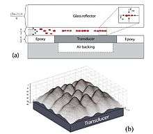
Figure 5 shows a side-view schematic of a microfluidic device. The glass reflector with etched fluidic channels is clamped to the PCB holding the transducer. Cells infused into the chip are trapped in the ultrasonic standing wave formed in the channel. The acoustic forces focus the cells into clusters in the center of the channel as illustrated in the inset. Since the trapping occurs close to the transducer surface, the actual trapping sites are given by the near-field pressure distribution as shown in the 3D image. Cells will be trapped in clusters around the local pressure minima creating different patterns depending on the number of cells trapped. The peaks in the graph correspond to the pressure minima.

Fig. 6: Traces of single cell manipulation

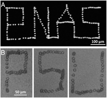
Manipulating single cells is important to many biological studies, such as in controlling the cellular microenvironment and isolating specific cells of interest. Acoustic tweezers have been demonstrated to manipulate each individual cell with micrometer-level resolution. Cells generally have a diameter of 10–20 μm. To meet the resolution requirements of manipulating single cells, short-wavelength acoustic waves should be employed. In this case, a surface acoustic wave (SAW) is preferred to a bulk acoustic wave (BAW), because it allows using shorter-wavelength acoustic waves (normally less than 200 μm).[22] Ding et al. reported a SSAW microdevice that is able to manipulate single cells with prescribed paths.[23] Figure 6 records a demonstration that the movement of single cells can be finely controlled with acoustic tweezers. The working principle of the device lies in the controlled movement of pressure nodes in an SSAW field. Ding et al. employed chirped interdigital transducers (IDTs) that are able to generate SSAWs with adjustable positions of pressure nodes by changing the input frequency. They also showed that the millimeter-sized microorganism C. elegan can be manipulated in the same manner. They also examined cell metabolism and proliferation after acoustic treatment, and found no significant differences compared to the control group, indicating the non-invasive nature of acoustic base manipulation. In addition to using chirped IDTs, phaseshift-based single particle/cell manipulation has also been reported.[24][25][26]

Sitters et al. have shown that acoustics can be used to manipulate single biomolecules such as DNA and proteins. This method, which the inventors call acoustic force spectroscopy, allows measuring the force response of single molecules. This is achieved by attaching small microspheres to the molecules at one side and attaching them to a surface at the other. By pushing the microspheres away from the surface with a standing acoustic wave the molecules are effectively stretched out.[27]

Polymer-dispersed liquid crystal (PDLC) displays can be switched from opaque to transparent using acoustic tweezers. A SAW-driven PDLC light shutter has been demonstrated by integrating a cured PDLC film and a pair of interdigital transducers (IDTs) onto a piezoelectric substrate.[28]

Acoustic tweezers provide a simple approach for tuneable nanowire patterning. In this approach, SSAWs are generated by interdigital transducers, which induced a periodic alternating current (AC) electric field on the piezoelectric substrate and consequently patterned metallic nanowires in suspension. The patterns could be deposited onto the substrate after the liquid evaporated. By controlling the distribution of the SSAW field, metallic nanowires are assembled into different patterns including parallel and perpendicular arrays. The spacing of the nanowire arrays could be tuned by controlling the frequency of the surface acoustic waves.[29]

While most acoustic tweezers are able to manipulate a large number of objects collectively,[22] a complementary function is to be able to manipulate a single particle within a cluster without moving adjacent objects. To achieve this goal, the acoustic trap must be localized spacially. A first approach consists in using highly focused acoustic beams.[30] Since many particles of interest are attracted to the nodes of an acoustic field and thus expelled from the focus point, some specific wave structures combining strong focalization but with a minimum of the pressure amplitude at the focal point (surrounded by a ring of intensity to create the trap) are required to trap this type of particle. These specific conditions are met by Bessel beams of topological order larger than zero, also called "acoustical vortices". With this kind of wave structures, the 3D selective manipulation of particles has been demonstrated with an array of transducers driven by programmable electronics.[31]

Fig. 7: 33 polystyrene microspheres arranged into a pattern using selective acoustic tweezers.

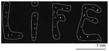
Compact flat acoustic tweezers based on spiral-shaped interdigital transducers have been proposed as an alternative to this complex array of transducer.[32] This type of device allows patterning dozens of microscopic particles on a microscope slide (see Figure 7). The selectivity was nevertheless limited since the acoustic vortex was only focused laterally and hence some spurious secondary rings of weaker could also trap particles.[32] Greater selectivity has been achieved by generating spherically focused acoustical vortices with a flat holographic transducer, combining underlying physical principles of Fresnel lenses in optics, the specificity of Bessel beam topology, and the principles of wave synthesis with IDTs.[33] These latter tweezers generate spherically focused acoustical vortices, and hold potential for 3D manipulation of particles. Alternatively, another approach to localize the acoustic energy relies on the use of nanosecond-scale pulsed fields to generate localized acoustic standing waves.[34]

References

- Gorkov, L. P.; Soviet Physics- Doklady, 1962, 6(9), 773-775.
- Nilsson, A; Petersson,F;Jonsson H.;Laurell T. Lab on a Chip .2004,4(2),131-135.
- S.-C. S. Lin, X. Mao, and T. J. Huang, Lab Chip, 2012, 12, 2766-2770.
- X. Ding, P. Li, S.-C. S. Lin, Z. S. Stratton, N. Nama, F. Guo, D. Slotcavage, X. Mao, J. Shi, F. Costanzo, and T. J. Huang, Lab on a Chip, 2013, 13, 3626-3649.
- Dion, J. L.; Malutta, A.; Cielo, P. (1982). "Ultrasonic Inspection Of Fiber Suspensions". Journal of the Acoustical Society of America. 72 (5): 1524–1526. Bibcode:1982ASAJ...72.1524D. doi:10.1121/1.388688.
- King, L. V.; Proc. R. Soc. London, Ser. A, 1934, 147(3), 212-240.
- Yosioka, K. and Kawasima, Y.; Acustica, 1955, 5(3), 167-173.
- Bruus, H.; Lab Chip, 2012, 12, 1014-1021.
- Weiser, M. A. H.; Apfel, R. E., and Neppiras, E. A.; Acustica, 1984, 56(2), 114-119.
- Laurell, T.; Petersson, F. and Nisson, A.; Chem. Soc. Rev., 2007, 36, 492-506.
- Sir Lighthill, J.; J. Sound Vib., 1978, 61(3), 391-418.
- Boluriann, S. and Morris, P. J.; Aeroacoustics, 2003, 2(3), 255-292.
- Bruus, H.; Lab Chip, 2012, 12, 20-28.
- J. Shi, H. Huang, Z. Stratton, Y. Huang and T. J. Huang, Lab Chip, 2009, 9, 3354-3359.
- J. Nam, H. Lim, D. Kim, and S. Shin, Lab on a Chip, 2011, 11, 3361-3364.
- Y. Ai, C. K. Sanders and B. L. Marrone, Anal. Chem., 2013, 85, 9126-9134.
- J. Nam, H. Lim, C. Kim, J. Yoon Kang and S. Shin, Biomicrofluidics, 2012, 6, 024120.
- J. Shi, X. Mao, D. Ahmed, A. Colletti, T. J. Huang, Lab Chip, 2008, 8, 221.
- J. Shi, S. Yazdi, S.-C. S. Lin, X. Ding, I-K. Chiang, K. Sharp, T. J. Huang, Lab Chip, 2011, 11, 2319.
- S. Li, X. Ding, F. Guo, Y. Chen, M. I. Lapsley, S.-C. S. Lin, L. Wang, J. P. McCoy, C. E. Cameron, T. J. Huang, Anal. Chem. 2013, 85, 5468.
- X. Ding, S.-C. S. Lin, M. I. Lapsley, S. Li, X. Guo, C. Y. K. Chan, I-K. Chiang, J. P. McCoy, T. J. Huang, Lab Chip, 2012, 12, 4228.
- M. Gedge and M. Hill, Lab on a Chip, 2012, 12, 2998-3007.
- X. Ding, S.-C. S. Lin, B. Kiraly, H. Yue, S. Li, I.-K. Chiang, J. Shi, S. J. Benkovic and T. J. Huang, Proceedings of the National Academy of Sciences, 2012, 109, 11105-11109.
- C. R. P. Courtney, C. E. M. Demore, H. Wu, A. Grinenko, P. D. Wilcox, S. Cochran, and B. W. Drinkwater, APPLIED PHYSICS LETTERS 104, 154103 (2014)
- L. Meng, F. Cai, J. Chen, L. Niu, Y. Li, J. Wu, and H. Zheng, Appl. Phys.Lett. 100, 173701 (2012).
- C. D. Wood, J. E. Cunningham, R. O'Rorke, C. Walti, E. H. Linfield, A. G. Davies, and S. D. Evans, Appl. Phys. Lett. 94, 054101 (2009).
- G. Sitters, D. Kamsma, G. Thalhammer, M. Ritch-Marte, E.J.G. Peterman, G.J.L. Wuite, Nature Methods 12. 47-50 (2015)
- Y. J. Liu, X. Ding, S.-C. S. Lin, J. Shi, I-K. Chiang, T. J. Huang, Adv. Mater. 2011, 23, 1656
- Y. Chen, X. Ding, S.-C. S. Lin, S. Yang, P.-H. Huang, N. Nama, Y. Zhao, A. A. Nawaz, F. Guo, W. Wang, Y. Gu, T. E. Mallouk, T. J. Huang, ACS Nano, 2013, 7, 3306.
- J. Lee, S.Y. Teh, A. Lee, H.H. Kim, C. Lee and K.K. Shung, Applied physics letters, 2009, 95(7), 073701.
- D. Baresch, J.L. Thomas, and R. Marchiano, Physical review letters, 2016, 116(2), 024301.
- A. Riaud, M. Baudoin, O. Bou Matar, L. Becerra, and J.L. Thomas, Physical Review Applied, 2017, 7(2), 024007.
- Baudoin, Michaël; Gerbedoen, Jean-Claude; Riaud, Antoine; Bou Matar, Olivier; Smagin, Nikolay; Thomas, Jean-Louis (2019). "Folding a focalized acoustical vortex on a flat holographic transducer: Miniaturized selective acoustical tweezers". Science Advances. 5: eaav1967. doi:10.1126/sciadv.aav1967.
- D.J. Collins, C. Devendran, Z. Ma, J.W. Ng, A. Neild and Y. Ai, Science Advances, 2016, 2(7), e1600089.
External links
- Fast acoustic tweezers — YouTube video illustrating how acoustic tweezers work